2 j j k Y AS Y a s Y a s a s j j T k - - PowerPoint PPT Presentation

2 j j k y as y a s y a s a s j j t k
SMART_READER_LITE
LIVE PREVIEW

2 j j k Y AS Y a s Y a s a s j j T k - - PowerPoint PPT Presentation

2 2 K K 2 j j k Y AS Y a s Y a s a s j j T k j 1 j k 2 k E a s k k Row k (NOT Does NOT depend column) of on the k-th matrix S dictionary column


slide-1
SLIDE 1

2 2 2 1 2 k k k K k j k k j T j K j j j

s a E s a s a Y s a Y AS Y        

 

 

Row ‘k’ (NOT column) of matrix S Does NOT depend

  • n the k-th

dictionary column

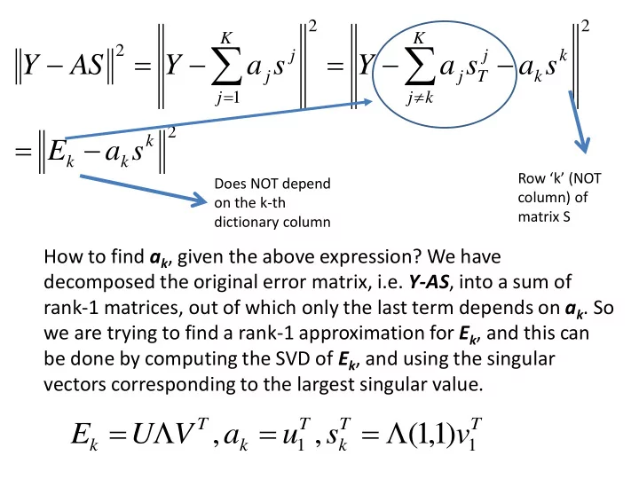
How to find ak, given the above expression? We have decomposed the original error matrix, i.e. Y-AS, into a sum of rank-1 matrices, out of which only the last term depends on ak. So we are trying to find a rank-1 approximation for Ek, and this can be done by computing the SVD of Ek, and using the singular vectors corresponding to the largest singular value.

T T k T k T k

v s u a V U E

1 1

) 1 , 1 ( , ,     

slide-2
SLIDE 2

Problem! The dictionary codes may no more be sparse! SVD does not have any in-built sparsity constraint in it! So, we proceed as follows:

} ) ( | {   i s i

k k

Consider the error matrix defined as follows:

T k k T k k k k F

V s U a V U E s a E AS Y

k k k k k k

1 1 , 2 , 2

) 1 , 1 ( , ) (        

      Considers only those columns of Y (i.e. only those data-points) that actually USE the k-th dictionary atom, effectively yielding a smaller matrix, of size p by |k| This update affects the sparse codes of only those data-points that used the k-th dictionary element, i.e. those that are part of ωk.

slide-3
SLIDE 3

http://www.cs.technion .ac.il/~elad/publications /journals/2004/32_KSV D_IEEE_TSP.pdf

slide-4
SLIDE 4

Application: Image Compression

  • Recall JPEG algorithm
  • It divides the image to be compressed into non-
  • verlapping patches of size 8 x 8.
  • It computes the 2D-DCT coefficients of each

patch, quantizes them and stores only the non- zero coefficients – using Huffman encoding.

  • KSVD can be used in image compression by

replacing the orthonormal 2D-DCT dictionary by an overcomplete dictionary trained on a database

  • f similar images.
slide-5
SLIDE 5

Application: Image Compression (Training Phase)

  • Training set for dictionary learning: a set of 11000

patches of size 8 x 8 – taken from a face image

  • database. Dictionary size K = 441 atoms

(elements).

  • OMP used in the sparse coding step during

training – stopping criterion is a fixed number of coefficients T0 = 10.

  • Over-complete Haar and DCT dictionaries – of

size 64 x 441 – and ortho-normal DCT basis of size 64 x 64 (JPEG), also used for comparison.

slide-6
SLIDE 6

http://www.cs.technion.ac.il/~elad/publication s/journals/2004/32_KSVD_IEEE_TSP.pdf

slide-7
SLIDE 7

Application: Image Compression (Testing Phase)

  • A lossy image compression algorithm is evaluated

using an ROC curve – the X axis contains the average number of bits (BPP) to store the signal.

  • The Y-axis is the compression error or PSNR.

Normally, the acceptable error e is fixed and the number of bits is calculated.

  • The test image is divided into non-overlapping

patches of size 8 x 8.

  • Each patch is projected onto the trained

dictionary and its sparse code is obtained using OMP given a fixed error e.

slide-8
SLIDE 8

Even if the error ‘e’ for the OMP was fixed, we need to compute the total MSE between the true and the compressed image. This is due to effects of quantization while storing the sparse coefficient values for each patch. http://www.cs.t echnion.ac.il/~el ad/publications/ journals/2004/3 2_KSVD_IEEE_TS P.pdf

slide-9
SLIDE 9

Application: Image Compression (Testing Phase)

  • The encoded image contains the following:
  • 1. Sparse-code coefficients for each patch and

the indices of each non-zero coefficient (in the dictionary).

  • 2. The number of coefficients used to represent

each patch (different patches will need different number of coefficients).

slide-10
SLIDE 10

Application: Image Compression (Testing Phase)

  • The average number of bits per pixel (BPP) is

calculated as:

pixels Q b coeffs patches a BPP # ) ( # #     

Number of bits required to store the number of coefficients for each patch Number of bits required to store the dictionary index for each coefficient Number of bits required to code each coefficient (quantization level) Sum total of the number of coefficients representing each patch Huffman encoding

slide-11
SLIDE 11

http://www.cs.technion.ac.il/~elad/publication s/journals/2004/32_KSVD_IEEE_TSP.pdf

slide-12
SLIDE 12

Application: Image Denoising

  • KSVD for denoising seeks to minimize the

following objective function:

2 , , 2 } { , ,

min arg }) { , , (

 

    

j i ij ij ij j i ij D X ij

X R D Y X D X

ij

    

Y = noisy image X = underlying clean image (to be estimated) ij = sparse dictionary coefficients for patch at location (i,j) D = dictionary Rij = matrix that extracts the patch xij from image X, i.e. xij = Rij X

slide-13
SLIDE 13

Application: Image Denoising

  • Note: The dictionary may be learned a priori from a

corpus of image patches. The patches from the noisy image can then be denoised by mere sparse coding.

  • The more preferable method is to train the dictionary

directly on the noisy image in tandem with the sparse coding step (as in the previous slide).

  • This avoids having to depend on the training set and

allows for tuning of the dictionary to the underlying image structure (as opposed to the structure of some

  • ther images).
slide-14
SLIDE 14

KSVD Algorithm for Denoising (Dictionary learned on the noisy image)

  • Set X = Y, D = overcomplete DCT
  • Until some “convergence” criterion is satisfied, repeat the

following: 1. Obtain the sparse codes for every patch (typically using OMP) as follows: 2. Perform the dictionary learning update typical for KSVD.

  • Estimate the final image X by averaging the reconstructed
  • verlapping patches, OR estimate X given D and ij:

2 2

s.t. min , ,    C D X R j i

ij ij ij

   ) ( ) ( min arg

1 2 2

  

       

 ij ij T ij ij ij T ij ij ij ij X

D R Y R R I X X R D Y X X     

slide-15
SLIDE 15

KSVD Algorithm for Denoising (Dictionary learned on the noisy image)

       30 set to ) ( ) ( min arg

1 2 2

  

       

 ij ij T ij ij ij T ij ij ij ij X

D R Y R R I X X R D Y X X

This equation is a mathematically rigorous way to show how X was reconstructed by averaging overlapping denoised patches together with the noisy image as well.

slide-16
SLIDE 16

Baseline for comparison: method by Portilla et al, “Image denoising using scale mixture of Gaussians in the wavelet domain”, IEEE TIP 2003. http://www.cs.technion.ac.il/~elad/publication s/journals/2005/KSVD_Denoising_IEEE_TIP.pdf

slide-17
SLIDE 17

http://www.cs.technion.ac.il/~elad/publication s/journals/2005/KSVD_Denoising_IEEE_TIP.pdf

slide-18
SLIDE 18

http://www.cs.technion.ac.il/~elad/Variou s/KSVD_Matlab_ToolBox.zip

slide-19
SLIDE 19

http://www.cs.technio n.ac.il/~elad/publicati

  • ns/journals/2005/KS

VD_Denoising_IEEE_TI P.pdf

slide-20
SLIDE 20

Application of KSVD: Filling in Missing Pixels

http://www.cs.technion.ac.il/~elad/publication s/journals/2004/32_KSVD_IEEE_TSP.pdf

slide-21
SLIDE 21

Application of KSVD: Filling in Missing Pixels

  • An over-complete dictionary is trained a priori on a set
  • f face images.
  • A test face image (not part of the training set) is

synthetically degraded by masking out 50 to 70 percent

  • f the pixels.
  • Patches from the degraded image are sparse coded by

projection onto the trained dictionary using OMP.

  • OMP is modified so that only the non-degraded pixels

are considered during any error computation (the dictionary elements are therefore appropriately re- scaled to unit norm).

slide-22
SLIDE 22

Application of KSVD: Filling in Missing Pixels

ISTA

  • r

OMP using determined codes Sparse priori

  • a

learned s.t. ~ }) ({ , , where ~ from s intensitie corrupted

  • non

the containing vector 1 ~ ) , ( location at image corrupted in patch 1

2 , 1 2

2 2

D T s Ds y s E R s R D R Ds y y P |P| y j i n y

ij j i ij ij ij ij K ij K n n P ij ij ij ij ij ij ij

              

  

slide-23
SLIDE 23

Application of KSVD: Filling in Missing Pixels

  • The patches are reconstructed in the following

manner:

ij ij

Ds y 

NOTE: Dictionary elements without masking!!

slide-24
SLIDE 24

Blind compressed sensing

  • In standard compressed sensing, we assume knowledge of

the basis (may be orthonormal or even overcomplete) in which the signal is sparse.

  • However this knowledge may not be available to us always.
  • For example, consider a remote sensing application with

compressive acquisitions of water bodies followed by forests over mountain ranges.

  • Images of the former are likely to be highly sparse in DCT

whereas the latter may not be – and another basis may serve a better purpose.

  • Blind compressed sensing is the task of inferring the signal

basis as well as the signal coefficients directly from the compressed data.

slide-25
SLIDE 25

Blind compressed sensing

  • Consider N signals and their compressive

measurements in the following form:

  • Our sparsity model for each signal is as

follows:

  • Combined model is:

n m R y R x R x y

m i n i n m i i i i i

       

, , , , 

K i K n i i

R R D D x   

  , ,

i i i i

D y     

slide-26
SLIDE 26

Blind compressed sensing

  • The objective function to be minimized is:
  • The algorithm for this is alternating in nature:

sparse coding assuming a fixed dictionary, and dictionary updates assuming sparse codes.

  • Sparse coding: OMP

1 , s.t. }) { , (

1 2

    

 k t k i N i i i i i

d d T D y D E    T D y E

i i i i i

   

2 1

s.t. ) (   

slide-27
SLIDE 27

Blind compressed sensing

  • The dictionary update is as follows:

    

      

          

N i ik k i k i N i ik k i il K k l l l i i N i il K l l i i k

d y d d y d y d E

1 2 ) ( 1 2 , 1 1 2 1

) (    

slide-28
SLIDE 28

Blind compressed sensing

  • Taking derivative w.r.t. dk and setting to 0

gives:

  • Repeat for other columns iteratively.

k i t i t k k i t i t k ik k k k ik N i k i t i N i ik i t i k ik N i ik k i k i t i

d d y d d d d y d d y                     

      

  

) ( 2 1 ) ( 1 1 2 1 ) (

/ ) ( 2     

This matrix will be invertible with probability 1 only if N is such that Nm >= n. Notice that it is important for every point to have a different sensing matrix, otherwise the dictionary cannot be inferred.

slide-29
SLIDE 29

Blind CS: Pseudocode

  • Start with a random dictionary, infer the

sparse codes for each data point.

  • Given the sparse codes, infer each column of

the dictionary keeping the others fixed. Infer the corresponding dictionary coefficients as well.

  • Repeat the previous two steps till a

convergence criterion is reached.