compression outline
play

Compression Outline Introduction : Lossy vs. Lossless, Benchmarks, - PowerPoint PPT Presentation

Compression Outline Introduction : Lossy vs. Lossless, Benchmarks, 15-583:Algorithms in the Real World Information Theory : Entropy, etc. Probability Coding : Huffman + Arithmetic Coding Data Compression II Arithmetic Coding Applications of


  1. Compression Outline Introduction : Lossy vs. Lossless, Benchmarks, … 15-583:Algorithms in the Real World Information Theory : Entropy, etc. Probability Coding : Huffman + Arithmetic Coding Data Compression II Arithmetic Coding Applications of Probability Coding : PPM + others – Integer implementation Lempel-Ziv Algorithms : LZ77, gzip, compress, ... Applications of Probability Coding Other Lossless Algorithms: Burrows-Wheeler – Run length coding: Fax ITU T4 Lossy algorithms for images: JPEG, fractals, ... – Residual coding: JPEG-LS Lossy algorithms for sound?: MP3, ... – Context Coding: PPM 15-853 Page1 15-853 Page2 Key points from last lecture 
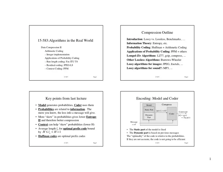
Encoding: Model and Coder Compress • Model generates probabilities, Coder uses them Model • Probabilities are related to information . The Static Part {p( s) | s ∈ S} more you know, the less info a message will give. Codeword Coder Dynamic |w| ≈ i M ( s ) • More “skew” in probabilities gives lower Entropy Part = -log p( s ) H and therefore better compression Message • Context can help “skew” probabilities (lower H) s ∈ S • Average length l a for optimal prefix code bound • The Static part of the model is fixed ≤ < + 1 by H l H • The Dynamic part is based on previous messages a • Huffman codes are optimal prefix codes The “optimality” of the code is relative to the probabilities. If they are not accurate, the code is not going to be efficient 15-853 Page3 15-853 Page4 1

  2. Decoding: Model and Decoder Adaptive Huffman Codes Uncompress Huffman codes can be made to be adaptive without Model completely recalculating the tree on each step. Static Part {p( s) | s ∈ S} • Can account for changing probabilities Codeword Decoder Dynamic • Small changes in probability, typically make small Part changes to the Huffman tree Message s ∈ S Used frequently in practice The probabilities {p(s) | s ∈ S} generated by the model need to be the same as generated in the encoder. Note : consecutive “messages” can be from a different message sets, and the probability distribution can change 15-853 Page5 15-853 Page6 Review some definitions Problem with Huffman Coding Message : an atomic unit that we will code. Consider a message with probability .999. The self information of this message is • Comes from a message set S = {s 1 ,…,s n } − log(. 999 ) = . 00144 with a probability distribution p(s). Probabilities must sum to 1. Set can be infinite. If we were to send a 1000 such message we might hope to use 1000*.0014 = 1.44 bits. • Also called symbol or character. Using Huffman codes we require at least one bit per Message sequence: a sequence of messages, message, so we would require 1000 bits. possibly each from its own probability distribution Code C(s) : A mapping from a message set to codewords , each of which is a string of bits 15-853 Page7 15-853 Page8 2

  3. Arithmetic Coding (message intervals) Arithmetic Coding: Introduction Allows “blending” of bits in a message sequence. Assign each probability distribution to an interval Only requires 3 bits for the example range from 0 (inclusive) to 1 (exclusive). Can bound total bits required based on sum of self e.g. 1.0 − 1 i c = .3 ∑ information: n ( ) ( ) f i = p j ∑ 0.7 2 l < + s i j = 1 b = .5 i = 1 f(a) = .0, f(b) = .2, f(c) = .7 Used in PPM, JPEG/MPEG (as option), DMM 0.2 a = .2 More expensive than Huffman coding, but integer 0.0 The interval for a particular message will be called implementation is not too bad. the message interval (e.g for b the interval is [.2,.7)) 15-853 Page9 15-853 Page10 Arithmetic Coding (sequence intervals) Arithmetic Coding: Encoding Example To code a message use the following: Coding the message sequence: bac = = + l f l l s f 0.7 1.0 0.3 1 1 − 1 − 1 i i i i c = .3 c = .3 c = .3 = = s p s s p 0.7 0.55 0.27 1 1 − 1 i i i b = .5 b = .5 b = .5 Each message narrows the interval by a factor of p i . n ∏ Final interval size: 0.2 0.3 0.21 = s p a = .2 a = .2 a = .2 0.0 n i 0.2 0.2 = 1 i The interval for a message sequence will be called The final interval is [.27,.3) the sequence interval 15-853 Page11 15-853 Page12 3

  4. Uniquely defining an interval Arithmetic Coding: Decoding Example Important property: The sequence intervals for Decoding the number .49, knowing the message is of distinct message sequences of length n will never length 3: overlap 0.7 0.55 1.0 Therefore: specifying any number in the final c = .3 c = .3 c = .3 0.49 interval uniquely determines the sequence. 0.7 0.55 0.475 0.49 0.49 Decoding is similar to encoding, but on each step b = .5 b = .5 b = .5 need to determine what the message value is and 0.2 0.3 0.35 then reduce interval a = .2 a = .2 a = .2 0.0 0.2 0.3 The message is bbc. 15-853 Page13 15-853 Page14 Representing an Interval Representing an Interval (continued) Binary fractional representation: Can view binary fractional numbers as intervals by considering all completions. e.g. . 75 . 11 = min max interval 1 3 / = . 0101 . 11 . 110 . 111 [. 7510 , . ) 11 16 / = . 1011 . 101 . 1010 . 1011 [. 625 75 ,. ) So how about just using the smallest binary We will call this the code interval. fractional representation in the sequence interval. e.g. [0,.33) = .01 [.33,.66) = .1 [.66,1) = .11 Lemma: If a set of code intervals do not overlap then the corresponding codes form a prefix code. But what if you receive a 1? Is the code complete? (Not a prefix code) 15-853 Page15 15-853 Page16 4

  5. Selecting the Code Interval RealArith Encoding and Decoding To find a prefix code find a binary fractional number RealArithEncode: whose code interval is contained in the sequence • Determine l and s using original recurrences interval. • Code using l + s/2 truncated to 1+  -log s  bits .79 .75 RealArithDecode: Sequence Interval Code Interval (.101) • Read bits as needed so code interval falls within a .625 .61 message interval, and then narrow sequence e.g. [0,.33) = .00 [.33,.66) = .100 [.66,1) = .11 interval. Can use l + s/2 truncated to • Repeat until n messages have been decoded .     − log( 2 ) = + − 1 log s s bits 15-853 Page17 15-853 Page18 Bound on Length Integer Arithmetic Coding Problem with RealArithCode is that operations on Theorem: For n messages with self information {s 1 ,…,s n } RealArithEncode will generate at most arbitrary precision real numbers is expensive. n ∑ s i bits. 2 + Key Ideas of integer version: = 1 i     n ∏ 1  log  1 log + − s = + −  p  • Keep integers in range [0..R) where R=2 k    i    i = 1 • Use rounding to generate integer interval   n ∑ 1 log = + − p   • Whenever sequence intervals falls into top, bottom i   i = 1 +   or middle half, expand the interval by factor of 2 n ∑ = 1 s   Integer Algorithm is an approximation i   = 1 i n ∑ < 2 + s i i = 1 15-853 Page19 15-853 Page20 5

  6. Integer Arithmetic Coding Integer Arithmetic (contracting) The probability distribution as integers l 1 = 0, s 1 = R = − + 1 • Probabilities as counts: s u l i i i e.g. c(1) = 11, c(2) = 7, c(3) = 30   ( ) / 1 u = l + s ⋅ f + s T − i i i i i • S is the sum of counts   / = + ⋅ l l s f T e.g. 48 (11+7+30) i i i i • Partial sums f as before: e.g. f(1) = 0, f(2) = 11, f(3) = 18 Require that R > 4S so that probabilities do not get rounded to zero 15-853 Page21 15-853 Page22 Integer Arithmetic (scaling) Applications of Probability Coding If l ≥ R/2 then ( in top half ) How do we generate the probabilities? Output 1 followed by m 0s Using character frequencies directly does not work m = 0 very well (e.g. 4.5 bits/char for text). Scale message interval by expanding by 2 Technique 1: transforming the data If u < R/2 then ( in bottom half ) • Run length coding (ITU Fax standard) Output 0 followed by m 1s m = 0 • Move-to-front coding (Used in Burrows-Wheeler) Scale message interval by expanding by 2 • Residual coding (JPEG LS) If l ≥ R/4 and u < 3R/4 then ( in middle half) Technique 2: using conditional probabilities Increment m • Fixed context (JBIG…almost) Scale message interval by expanding by 2 • Partial matching (PPM) 15-853 Page23 15-853 Page24 6

Download Presentation
Download Policy: The content available on the website is offered to you 'AS IS' for your personal information and use only. It cannot be commercialized, licensed, or distributed on other websites without prior consent from the author. To download a presentation, simply click this link. If you encounter any difficulties during the download process, it's possible that the publisher has removed the file from their server.

Recommend


More recommend