Combining probabilities with log-linear pooling : application to - PowerPoint PPT Presentation

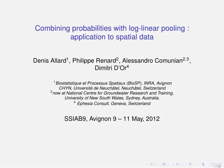
Combining probabilities with log-linear pooling : application to spatial data Denis Allard 1 , Philippe Renard 2 , Alessandro Comunian 2 , 3 , Dimitri D’Or 4 1 Biostatistique et Processus Spatiaux (BioSP), INRA, Avignon CHYN, Université de Neuchâtel, Neuchâtel, Switzerland 3 now at National Centre for Groundwater Research and Training, University of New South Wales, Sydney, Australia. 4 Ephesia Consult, Geneva, Switzerland SSIAB9, Avignon 9 – 11 May, 2012 1 / 25

General framework ◮ Consider discrete events : A ∈ A = { A 1 , . . . , A K } = A . ◮ We know conditional probabilities P ( A | D i ) = P i ( A ) , where the D i s come from different sources of information. ◮ We include the possibility of a prior probability, P 0 ( A ) . ◮ Example : ◮ A = soil type ◮ ( D i ) = { remote sensing information, soil samples, a priori pattern,... } Purpose To provide an approximation of the probability P ( A | D 1 , . . . , D n ) on the basis of the simultaneous knowledge of P 0 ( A ) and the n conditional probabilities P ( A | D i ) = P i ( A ) , without the knowledge of a joint model : P ( A | D 0 , . . . , D n ) ≈ P G ( P ( A | D 0 ) , . . . , P ( A | D n )) . (1) 2 / 25

General framework ◮ Consider discrete events : A ∈ A = { A 1 , . . . , A K } = A . ◮ We know conditional probabilities P ( A | D i ) = P i ( A ) , where the D i s come from different sources of information. ◮ We include the possibility of a prior probability, P 0 ( A ) . ◮ Example : ◮ A = soil type ◮ ( D i ) = { remote sensing information, soil samples, a priori pattern,... } Purpose To provide an approximation of the probability P ( A | D 1 , . . . , D n ) on the basis of the simultaneous knowledge of P 0 ( A ) and the n conditional probabilities P ( A | D i ) = P i ( A ) , without the knowledge of a joint model : P ( A | D 0 , . . . , D n ) ≈ P G ( P ( A | D 0 ) , . . . , P ( A | D n )) . (1) 2 / 25

Outline ◮ Mathematical properties ◮ Pooling formulas ◮ Scores and calibration ◮ Maximum likelihood ◮ Some results 3 / 25

Some mathematical properties Convexity An aggregation operator P G verifying P G ∈ [ min { P 1 , . . . , P n } , max { P 1 , . . . , P n } ] , (2) is convex. Unanimity preservation An aggregation operator P G verifying P G = p when P i = p for i = 1 , . . . , n is said to preserve unanimity. Convexity implies unanimity preservation. In general, convexity is not necessarily a desirable property. 4 / 25

Some mathematical properties Convexity An aggregation operator P G verifying P G ∈ [ min { P 1 , . . . , P n } , max { P 1 , . . . , P n } ] , (2) is convex. Unanimity preservation An aggregation operator P G verifying P G = p when P i = p for i = 1 , . . . , n is said to preserve unanimity. Convexity implies unanimity preservation. In general, convexity is not necessarily a desirable property. 4 / 25

Some mathematical properties External Bayesianity An aggregation operator is said to be external Bayesian if the operation of updating the probabilities with the likelihood L commutes with the aggregation operator, that is if P G ( P L 1 , . . . , P L n )( A ) = P L G ( P 1 , . . . , P n )( A ) . (3) ◮ It should not matter whether new information arrives before or after pooling ◮ Equivalent to the weak likelihood ratio property in Bordley (1982). ◮ Very compelling property, both from a theoretical point of view and from an algorithmic point of view. Imposing this property leads to a very specific class of pooling operators. 5 / 25

Some mathematical properties External Bayesianity An aggregation operator is said to be external Bayesian if the operation of updating the probabilities with the likelihood L commutes with the aggregation operator, that is if P G ( P L 1 , . . . , P L n )( A ) = P L G ( P 1 , . . . , P n )( A ) . (3) ◮ It should not matter whether new information arrives before or after pooling ◮ Equivalent to the weak likelihood ratio property in Bordley (1982). ◮ Very compelling property, both from a theoretical point of view and from an algorithmic point of view. Imposing this property leads to a very specific class of pooling operators. 5 / 25

Some mathematical properties 0/1 forcing An aggregation operator which returns P G ( A ) = 0 if P i ( A ) = 0 for some i = 1 , . . . , n is said to enforce a certainty effect, a property also called the 0/1 forcing property. 6 / 25

Linear pooling Linear Pooling n � P G ( A ) = w i P i ( A ) , (4) i = 0 where the w i are positive weights verifying � n i = 0 w i = 1 ◮ Convex ⇒ preserves unanimity. ◮ Neither verify external bayesianity, nor 0/1 forcing ◮ Cannot achieve calibration (Ranjan and Geniting, 2010). Ranjan and Gneiting (2010) proposed a Beta transformation of the linear pooling. Parameters are estimated via ML. 7 / 25

Log-linear pooling Log-linear pooling A log-linear pooling operator is a linear operator of the logarithms of the probabilities : n � ln P G ( A ) = ln Z + w i ln P i ( A ) , (5) i = 0 or equivalently n � P i ( A ) w i , P G ( A ) ∝ (6) i = 0 where Z is a normalizing constant. ◮ Non Convex but preserves unanimity if � n i = 0 = 1 ◮ Verifies 0/1 forcing ◮ Verifies external bayesianity (Genest and Zidek, 1986) 8 / 25

Generalized log-linear pooling Theorem (Genest and Zidek, 1986) The only pooling operator P G depending explicitly on A and verifying external Bayesianity is n P G ( A ) ∝ ν ( A ) P 0 ( A ) 1 − � n � P i ( A ) w i . i = 1 w i (7) i = 1 No restriction on the w i s ; verifies external Bayesianity and 0/1 forcing. 9 / 25

Generalized log-linear pooling n P G ( A ) ∝ ν ( A ) P 0 ( A ) 1 − � n � P i ( A ) w i . i = 1 w i (8) i = 1 The sum S w = � n i = 1 w i plays an important role. Suppose that P i = p for each i = 1 , . . . , n . ◮ If S w = 1, the prior probability P 0 is filtered out. Then, P G = p and unanimity is preserved ◮ if S w > 1, the prior probability has a negative weight and P G will always be further from P 0 than p ◮ S w < 1, the converse holds 10 / 25

Maximum entropy approach Proposition The pooling formula P G maximizing the entropy subject to the following univariate and bivariate constraints P G ( P 0 )( A ) = P 0 ( A ) and P G ( P 0 , P i )( A ) = P ( A | D i ) for i = 1 , . . . , n is P 0 ( A ) 1 − n � n i = 1 P i ( A ) P G ( P 1 , . . . , P n )( A ) = i = 1 P i ( A ) . (9) A ∈A P 0 ( A ) 1 − n � n � i.e. it is a log-linear formula with w i = 1, for all i = 1 , . . . , n . Proposed in Allard (2011) for non parametric spatial prediction of soil type categories. { Max. Ent. } ⊂ { Log linear pooling } ⊂ { Gen. log-linear pooling } . 11 / 25

Maximum Entropy for spatial prediction 12 / 25

Maximum Entropy for spatial prediction 13 / 25

Maximum Entropy for spatial prediction 14 / 25

Estimating the weights Maximum entropy is parameter free. For all other models, how do we estimate the parameters ? We will minimize scores Quadratic or Brier score The quadratic or Brier score (Brier, 1950) is defined by K ( δ jk − P G ( j )) 2 � S ( P G , A k ) = (10) j = 1 Minimizing Brier score ⇔ minimizing Euclidien distance. Logarithmic score The logarithmic score corresponds to S ( P G , A k ) = ln P G ( k ) (11) Maximizing the logarithmic score ⇔ minimizing KL distance. 15 / 25

Estimating the weights Maximum entropy is parameter free. For all other models, how do we estimate the parameters ? We will minimize scores Quadratic or Brier score The quadratic or Brier score (Brier, 1950) is defined by K ( δ jk − P G ( j )) 2 � S ( P G , A k ) = (10) j = 1 Minimizing Brier score ⇔ minimizing Euclidien distance. Logarithmic score The logarithmic score corresponds to S ( P G , A k ) = ln P G ( k ) (11) Maximizing the logarithmic score ⇔ minimizing KL distance. 15 / 25

Estimating the weights Maximum entropy is parameter free. For all other models, how do we estimate the parameters ? We will minimize scores Quadratic or Brier score The quadratic or Brier score (Brier, 1950) is defined by K ( δ jk − P G ( j )) 2 � S ( P G , A k ) = (10) j = 1 Minimizing Brier score ⇔ minimizing Euclidien distance. Logarithmic score The logarithmic score corresponds to S ( P G , A k ) = ln P G ( k ) (11) Maximizing the logarithmic score ⇔ minimizing KL distance. 15 / 25

Maximum likelihood estimation Maximizing the logarithmic score ⇔ maximizing the log-likelihood. Let is consider M repetitions of a random experiment. For m = 1 , . . . , M : ◮ conditional probabilities P ( m ) ( A k ) i ◮ aggregated probabilities P ( m ) G ( A k ) ◮ Y ( m ) = 1 if the outcome is A k and Y ( m ) = 0 otherwise k k M K � n n � � � Y ( m ) � � w i ln P ( m ) L ( w ,ν ν ν ) = ln ν k + ( 1 − w i ) ln P 0 , k + k i , k m = 1 k = 1 i = 1 i = 1 � K M n � 1 − � n i = 1 w i ( P ( m ) � � � i , k ) w i − ln ν k P (12) . 0 , k m = 1 k = 1 i = 1 16 / 25

Calibration Calibration The aggregated probability P G ( A ) is said to be calibrated if P ( Y k | P G ( A k )) = P G ( A k ) , k = 1 , . . . , K (13) Theorem (Ranjan and Gneiting, 2010) Linear pooling cannot be calibrated. Theorem (Allard et al. , 2012) If there exists a calibrated log-linear pooling, it is, asymptotically, the (generalized) log-linear pooling with parameters estimated from maximum likelihood. 17 / 25