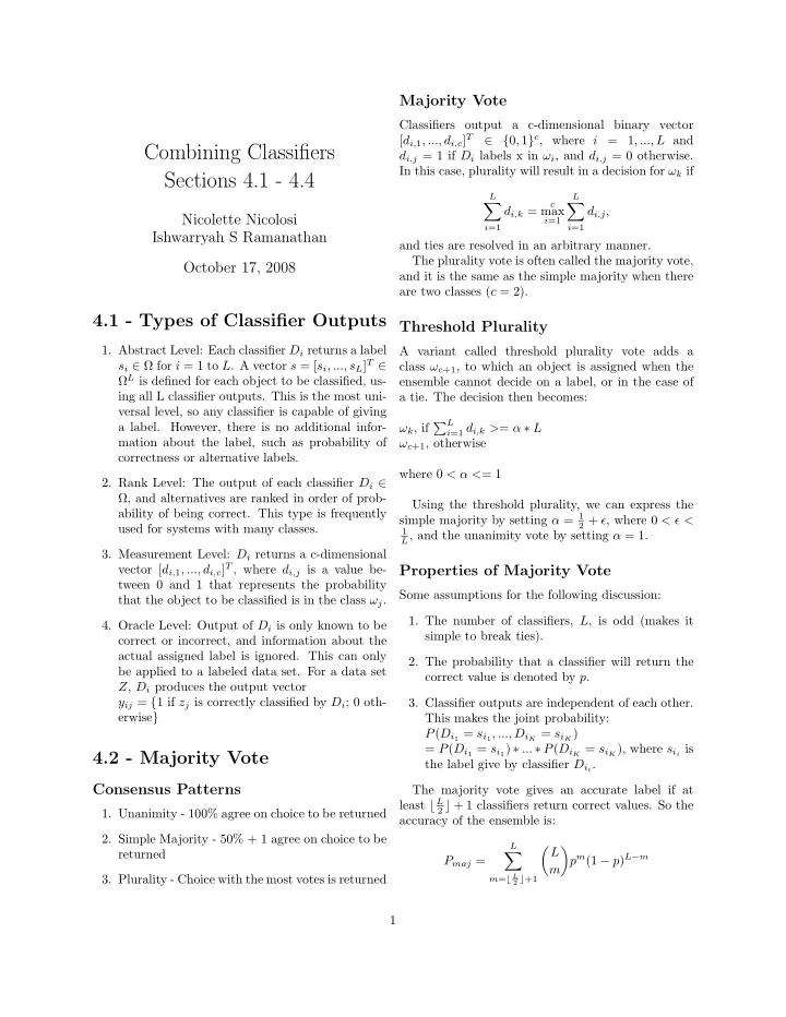
Combining Classifiers d i,j = 1 if D i labels x in i , and d i,j = 0 - PDF document

Majority Vote Classifiers output a c-dimensional binary vector [ d i, 1 , ..., d i,c ] T ∈ { 0 , 1 } c , where i = 1 , ..., L and Combining Classifiers d i,j = 1 if D i labels x in ω i , and d i,j = 0 otherwise. In this case, plurality will result in a decision for ω k if Sections 4.1 - 4.4 L L c � � d i,k = max d i,j , Nicolette Nicolosi i =1 i =1 i =1 Ishwarryah S Ramanathan and ties are resolved in an arbitrary manner. The plurality vote is often called the majority vote, October 17, 2008 and it is the same as the simple majority when there are two classes ( c = 2). 4.1 - Types of Classifier Outputs Threshold Plurality 1. Abstract Level: Each classifier D i returns a label A variant called threshold plurality vote adds a s i ∈ Ω for i = 1 to L . A vector s = [ s i , ..., s L ] T ∈ class ω c +1 , to which an object is assigned when the Ω L is defined for each object to be classified, us- ensemble cannot decide on a label, or in the case of ing all L classifier outputs. This is the most uni- a tie. The decision then becomes: versal level, so any classifier is capable of giving ω k , if � L a label. However, there is no additional infor- i =1 d i,k > = α ∗ L mation about the label, such as probability of ω c +1 , otherwise correctness or alternative labels. where 0 < α < = 1 2. Rank Level: The output of each classifier D i ∈ Ω, and alternatives are ranked in order of prob- Using the threshold plurality, we can express the ability of being correct. This type is frequently simple majority by setting α = 1 2 + ǫ , where 0 < ǫ < used for systems with many classes. 1 L , and the unanimity vote by setting α = 1. 3. Measurement Level: D i returns a c-dimensional vector [ d i, 1 , ..., d i,c ] T , where d i,j is a value be- Properties of Majority Vote tween 0 and 1 that represents the probability Some assumptions for the following discussion: that the object to be classified is in the class ω j . 1. The number of classifiers, L , is odd (makes it 4. Oracle Level: Output of D i is only known to be simple to break ties). correct or incorrect, and information about the actual assigned label is ignored. This can only 2. The probability that a classifier will return the be applied to a labeled data set. For a data set correct value is denoted by p . Z , D i produces the output vector y ij = { 1 if z j is correctly classified by D i ; 0 oth- 3. Classifier outputs are independent of each other. erwise } This makes the joint probability: P ( D i 1 = s i 1 , ..., D i K = s i K ) = P ( D i 1 = s i 1 ) ∗ ... ∗ P ( D i K = s i K ) , where s i i is 4.2 - Majority Vote the label give by classifier D i i . Consensus Patterns The majority vote gives an accurate label if at least ⌊ L 2 ⌋ + 1 classifiers return correct values. So the 1. Unanimity - 100% agree on choice to be returned accuracy of the ensemble is: 2. Simple Majority - 50% + 1 agree on choice to be L � L � returned � p m (1 − p ) L − m P maj = m 3. Plurality - Choice with the most votes is returned m = ⌊ L 2 ⌋ +1 1

Condorcet Jury Theorem cases are ”the pattern of success” and ”the pattern of failure,” respectively. The Condorcet Jury Theorem supports the intuitive expectation that improvements over the individual Patterns of Success and Failure accuracy p will only occur when p is larger than 0.5. p i is an individual accuracy for classifier D i . Let l = 1. If p > 0 . 5, P maj is monotonically increasing ⌊ L 2 ⌋ . (strictly increasing) and P maj → 1 as L → ∞ . A pattern is a success pattern if the: 1. Probability of any combination of ⌊ L 2. If p < 0 . 5, P maj is monotonically decreasing and 2 +1 ⌋ correct P maj → 0 as L → ∞ and ⌊ L 2 ⌋ incorrect votes is α 2. Probability of all L votes being incorrect is γ 3. If p = 0 . 5, P maj = 0 . 5 for any L . 3. Probability of any other combination is 0 Limits on Majority Vote The pattern of success occurs when exactly ⌊ L 2 ⌋ +1 D = { D 1 , D 2 , D 3 } is an ensemble of three classifiers, votes are correct. This results in using the minimum each of which has the same probability of correctly number of votes required, without wasting votes. In this case, classifying a sample ( p = 0 . 6). All combinations dis- � L � tributing 10 elements into the 8 combinations of out- P maj = α, puts can be represented if we represent each classifier l + 1 output as either a 0 or a 1. For example, 101 would and the pattern of success is possible when represent the case where the first and third, but not 1 P maj ≤ 1, so α ≤ l +1 ). Using these definitions, we ( L the second, classifiers correctly labeled a certain num- � L − 1 � can rewrite the accuracy p = α . Substituting ber of samples X. 1 this rewritten definition for p , we obtain: l + 1 = 2 pL pL P maj = L + 1 If P maj ≤ 1 and p ≤ L +1 2 L , then: � 1 , 2 pL � P maj = min L + 1 A pattern is a failure pattern if the: 1. Probability of any combination of ⌊ L 2 ⌋ correct and ⌊ L 2 ⌋ + 1 incorrect votes is β 2. Probability of all L votes being incorrect is δ 3. Probability of any other combination is 0 The pattern of failure occurs when exactly l out of L classifiers are correct. In this case, � L � In the table, there is a case where the majority vote P maj = δ = 1 − β l is correct 90 percent of the time. This is unlikely, but it is an improvement over the individual rate p = 0 . 6. The accuracy p can be rewritten using P maj and α : There is also a case in which the majority vote is cor- rect only 40 percent of the time, which is worse than � L − 1 � p = δ + β the individual rate. These best and worst possible l − 1 2

4.4 - Naive Bayes Combination These equations can be combined to give: Naive Bayes combination assumes that classifiers are P maj = pL − 1 = (2 p − 1)( L + 1) mutually independent given a class label. In practice, l + 1 L + 1 the classifiers are frequently dependent upon each other in spite of this assumption. Interestingly, Matan’s Upper and Lower Bounds the Bayes classifier is still often fairly accurate and efficient in these situations. The probability that D j A classifier D i has accuracy p i , and L classifiers are labels x in class s j ∈ Ω is P ( s j ). The conditional ordered so that p 1 ≤ p 2 ≤ p 3 , . . . , ≤ p L . Let k = independence is then: l + 1 = ( L +1) and m = 1 , 2 , 3 , . . . , k . 2 The upper bound is the same as the pattern of L � success: P ( s | ω k ) = P ( s 1 , s 2 , ..., s L | ω k ) = P ( s i | ω k ) i =1 � � � � � From this equation, it follows that the posterior max P maj = min 1 , k, k − 1 , . . . , 1 probability necessary to label x is: where � 1 � L − k + m P ( ω k | s ) = P ( ω k ) P ( s | ω k ) � � m = p i m P ( s ) i =1 P ( ω k | s ) = P ( ω k ) � L The lower bound is the same as the pattern of i =1 P ( s i | ω k ) , failure: P ( s ) for k = 1 , ..., c min P maj = max { 0 , ξ ( k ) , ξ ( k − 1) , . . . , ξ (1) } The denominator is ignored because it is irrelevant where for ω k , so the support for ω k is: � 1 L � p i − ( L − k ) � ξ ( m ) = L m m � i = k − m +1 µ k ( x ) ∝ P ( ω k ) P ( s i | ω k ) i =1 4.3 - Weighted Majority Vote One way to select weights Consider an ensemble of L independent classifiers. Adding weights to the majority vote is an attempt to D i denotes a classifier and p i denotes its associated favor the more accurate classifiers in making the final individual accuracy. The accuracy of the ensemble is decision. Representing label outputs in the following maximized by assigning weights: way uses them as ”degrees of support” for the classes: p i b i ∝ log � 1 1 − p i if D i labels x in ω j , d i,j = For each classifier D i , a c by c confusion matrix 0 otherwise . CM i defined by applying D i to the training set. The (k,s)th entry of the matrix cm i k,s represents the num- The discriminant function for class ω j is: ber of elements that belong to ω k that were assigned the ω s by D i . This confusion matrix can be used to L estimate the probability P ( s i | ω k ). Specifically, � g j ( x ) = b i d i,j cm i i =1 k,s P ( s i | ω k ) = N k where b i is a coefficient for D i . The discriminant The estimated posterior probability for ω s is N k function is the sum of coefficients for classifiers in the N . ensemble for which the output on x is ω j . With this, we can rewrite the support equation for 3

ω k : � L � 1 � cm i µ k ( x ) ∝ k,s i N L − 1 k i =1 If the estimate for P ( s i | ω k ) is zero, µ k ( x ) is nulli- fied. 4