Combinatorial Reciprocity Theorems Matthias Beck Based on joint - PowerPoint PPT Presentation

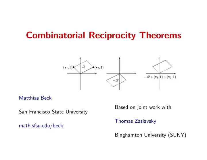
Combinatorial Reciprocity Theorems Matthias Beck Based on joint work with San Francisco State University Thomas Zaslavsky math.sfsu.edu/beck Binghamton University (SUNY)

“In mathematics you don’t understand things. You just get used to them.” John von Neumann (1903–1957) Combinatorial Reciprocity Theorems Matthias Beck 2

The Theme Combinatorics counting function depending on k ∈ Z > 0 polynomial p ( k ) What is p (0) ? p ( − 1) ? p ( − 2) ? Combinatorial Reciprocity Theorems Matthias Beck 3

The Theme Combinatorics counting function depending on k ∈ Z > 0 polynomial p ( k ) What is p (0) ? p ( − 1) ? p ( − 2) ? Two-for-one charm of combinatorial reciprocity theorems ◮ “Big picture” motivation: understand/classify these polynomials ◮ Combinatorial Reciprocity Theorems Matthias Beck 3

Chromatic Polynomials of Graphs G = ( V, E ) — graph (without loops) k -coloring of G — mapping x ∈ { 1 , 2 , . . . , k } V Combinatorial Reciprocity Theorems Matthias Beck 4

Chromatic Polynomials of Graphs G = ( V, E ) — graph (without loops) Proper k -coloring of G — x ∈ { 1 , 2 , . . . , k } V such that x i � = x j if ij ∈ E χ G ( k ) := # ( proper k -colorings of G ) Example: • ✡ ❏ ✡ ❏ ✡ ❏ ✡ ❏ ✡ ❏ ✡ ❏ ✡ ❏ • • ✡ ❏ Combinatorial Reciprocity Theorems Matthias Beck 4

Chromatic Polynomials of Graphs G = ( V, E ) — graph (without loops) Proper k -coloring of G — x ∈ { 1 , 2 , . . . , k } V such that x i � = x j if ij ∈ E χ G ( k ) := # ( proper k -colorings of G ) Example: • ✡ ❏ ✡ ❏ ✡ ❏ χ K 3 ( k ) = k · · · ✡ ❏ ✡ ❏ ✡ ❏ ✡ ❏ • • ✡ ❏ Combinatorial Reciprocity Theorems Matthias Beck 4

Chromatic Polynomials of Graphs G = ( V, E ) — graph (without loops) Proper k -coloring of G — x ∈ { 1 , 2 , . . . , k } V such that x i � = x j if ij ∈ E χ G ( k ) := # ( proper k -colorings of G ) Example: • ✡ ❏ ✡ ❏ ✡ ❏ χ K 3 ( k ) = k ( k − 1) · · · ✡ ❏ ✡ ❏ ✡ ❏ ✡ ❏ • • ✡ ❏ Combinatorial Reciprocity Theorems Matthias Beck 4

Chromatic Polynomials of Graphs G = ( V, E ) — graph (without loops) Proper k -coloring of G — x ∈ { 1 , 2 , . . . , k } V such that x i � = x j if ij ∈ E χ G ( k ) := # ( proper k -colorings of G ) Example: • ✡ ❏ ✡ ❏ ✡ ❏ χ K 3 ( k ) = k ( k − 1)( k − 2) ✡ ❏ ✡ ❏ ✡ ❏ ✡ ❏ • • ✡ ❏ Combinatorial Reciprocity Theorems Matthias Beck 4

Chromatic Polynomials of Graphs • ✡ ❏ ✡ ❏ ✡ ❏ χ K 3 ( k ) = k ( k − 1)( k − 2) ✡ ❏ ✡ ❏ ✡ ❏ ✡ ❏ • • ✡ ❏ Theorem (Birkhoff 1912, Whitney 1932) χ G ( k ) is a polynomial in k . Combinatorial Reciprocity Theorems Matthias Beck 5

Chromatic Polynomials of Graphs • ✡ ❏ ✡ ❏ ✡ ❏ χ K 3 ( k ) = k ( k − 1)( k − 2) ✡ ❏ ✡ ❏ ✡ ❏ ✡ ❏ • • ✡ ❏ Theorem (Birkhoff 1912, Whitney 1932) χ G ( k ) is a polynomial in k . | χ K 3 ( − 1) | = 6 counts the number of acyclic orientations of K 3 . Combinatorial Reciprocity Theorems Matthias Beck 5

Chromatic Polynomials of Graphs • ✡ ❏ ✡ ❏ ✡ ❏ χ K 3 ( k ) = k ( k − 1)( k − 2) ✡ ❏ ✡ ❏ ✡ ❏ ✡ ❏ • • ✡ ❏ Theorem (Birkhoff 1912, Whitney 1932) χ G ( k ) is a polynomial in k . | χ K 3 ( − 1) | = 6 counts the number of acyclic orientations of K 3 . Theorem (Stanley 1973) ( − 1) | V | χ G ( − k ) equals the number of pairs ( α, x ) consisting of an acyclic orientation α of G and a compatible k -coloring x . In particular, ( − 1) | V | χ G ( − 1) equals the number of acyclic orientations of G . Combinatorial Reciprocity Theorems Matthias Beck 5

If you get bored. . . Show that the coefficients of χ G alternate in sign. [old news] ◮ Show that the absolute values of the coefficients form a unimodal ◮ sequence. [J. Huh, arXiv:1008.4749 ] Show that χ G (4) > 0 for any planar graph G . [impressive with or ◮ without a computer] Show that χ G has no real root ≥ 4 . [open] ◮ Classify chromatic polynomials. [wide open] ◮ Combinatorial Reciprocity Theorems Matthias Beck 6

Hyperplane Arrangements H ⊂ R d — arrangement of affine hyperplanes L ( H ) — all nonempty intersections of hyperplanes in H  if F = R d 1   M¨ obius function µ ( F ) := � − µ ( G ) otherwise   G � F � µ ( F ) k dim F Characteristic polynomial p H ( k ) := F ∈L ( H ) • � ❅ ❅ � ❅ ❅ � ❅ ❅ � ❅ ❅ � ❅ ✏✏✏✏✏✏✏✏✏✏✏✏✏✏✏✏✏✏✏✏ ❅ � ❅ ❅ ❤❤❤❤❤❤❤❤❤❤❤❤❤❤❤❤❤❤❤❤❤❤❤ • � • ❅ • ❅ ❅ � • ❅ ❅ � ❅ ❅ � ❅ ❅ � ❅ ❅ � ❅ ❅ � ❅ ❅ • R 2 � ❅ ❅ Combinatorial Reciprocity Theorems Matthias Beck 7

Hyperplane Arrangements H ⊂ R d — arrangement of affine hyperplanes L ( H ) — all nonempty intersections of hyperplanes in H  if F = R d 1   M¨ obius function µ ( F ) := � − µ ( F ) otherwise   G � F � µ ( F ) k dim F Characteristic polynomial p H ( k ) := F ∈L ( H ) • � ❅ ❅ � ❅ ❅ � ❅ ❅ � ❅ ❅ � ❅ ✏✏✏✏✏✏✏✏✏✏✏✏✏✏✏✏✏✏✏✏ ❅ � ❅ ❅ ❤❤❤❤❤❤❤❤❤❤❤❤❤❤❤❤❤❤❤❤❤❤❤ • � • ❅ • ❅ ❅ � • ❅ ❅ � ❅ ❅ � ❅ ❅ � ❅ ❅ � ❅ ❅ � ❅ ❅ • R 2 � ❅ 1 ❅ Combinatorial Reciprocity Theorems Matthias Beck 7

Hyperplane Arrangements H ⊂ R d — arrangement of affine hyperplanes L ( H ) — all nonempty intersections of hyperplanes in H  if F = R d 1   M¨ obius function µ ( F ) := � − µ ( F ) otherwise   G � F � µ ( F ) k dim F Characteristic polynomial p H ( k ) := F ∈L ( H ) • � ❅ ❅ � ❅ ❅ � ❅ ❅ � ❅ ❅ � ❅ ✏✏✏✏✏✏✏✏✏✏✏✏✏✏✏✏✏✏✏✏ ❅ � ❅ ❅ ❤❤❤❤❤❤❤❤❤❤❤❤❤❤❤❤❤❤❤❤❤❤❤ • − 1 � • ❅ • ❅ ❅ � • ❅ ❅ � ❅ ❅ � ❅ ❅ � ❅ ❅ � ❅ ❅ � ❅ ❅ • R 2 � ❅ 1 ❅ Combinatorial Reciprocity Theorems Matthias Beck 7

Hyperplane Arrangements H ⊂ R d — arrangement of affine hyperplanes L ( H ) — all nonempty intersections of hyperplanes in H  if F = R d 1   M¨ obius function µ ( F ) := � − µ ( F ) otherwise   G � F � µ ( F ) k dim F Characteristic polynomial p H ( k ) := F ∈L ( H ) • � ❅ ❅ � ❅ ❅ � ❅ ❅ � ❅ ❅ � ❅ ✏✏✏✏✏✏✏✏✏✏✏✏✏✏✏✏✏✏✏✏ ❅ � ❅ ❅ ❤❤❤❤❤❤❤❤❤❤❤❤❤❤❤❤❤❤❤❤❤❤❤ • − 1 � •− 1 ❅ •− 1 ❅ ❅ � • ❅ ❅ � ❅ ❅ � ❅ ❅ � ❅ ❅ � ❅ ❅ � ❅ ❅ • R 2 � ❅ 1 ❅ Combinatorial Reciprocity Theorems Matthias Beck 7

Hyperplane Arrangements H ⊂ R d — arrangement of affine hyperplanes L ( H ) — all nonempty intersections of hyperplanes in H  if F = R d 1   M¨ obius function µ ( F ) := � − µ ( F ) otherwise   G � F � µ ( F ) k dim F Characteristic polynomial p H ( k ) := F ∈L ( H ) • 2 � ❅ ❅ � ❅ ❅ � ❅ ❅ � ❅ ❅ � ❅ ✏✏✏✏✏✏✏✏✏✏✏✏✏✏✏✏✏✏✏✏ ❅ � ❅ ❅ ❤❤❤❤❤❤❤❤❤❤❤❤❤❤❤❤❤❤❤❤❤❤❤ • − 1 � •− 1 ❅ •− 1 ❅ ❅ � • ❅ ❅ � ❅ ❅ � ❅ ❅ � ❅ ❅ � ❅ ❅ � ❅ ❅ • R 2 � ❅ 1 ❅ Combinatorial Reciprocity Theorems Matthias Beck 7

Hyperplane Arrangements H ⊂ R d — arrangement of affine hyperplanes L ( H ) — all nonempty intersections of hyperplanes in H  if F = R d 1   M¨ obius function µ ( F ) := � − µ ( F ) otherwise   G � F µ ( F ) k dim F = k 2 − 3 k + 2 � Characteristic polynomial p H ( k ) := F ∈L ( H ) • 2 � ❅ ❅ � ❅ ❅ � ❅ ❅ � ❅ ❅ � ❅ ✏✏✏✏✏✏✏✏✏✏✏✏✏✏✏✏✏✏✏✏ ❅ � ❅ ❅ ❤❤❤❤❤❤❤❤❤❤❤❤❤❤❤❤❤❤❤❤❤❤❤ • − 1 � •− 1 ❅ •− 1 ❅ ❅ � • ❅ ❅ � ❅ ❅ � ❅ ❅ � ❅ ❅ � ❅ ❅ � ❅ ❅ • R 2 � ❅ 1 ❅ Combinatorial Reciprocity Theorems Matthias Beck 7

Hyperplane Arrangements • 2 � ❅ ❅ � ❅ ❅ � ❅ ❅ � ❅ ❅ ✏✏✏✏✏✏✏✏✏✏✏✏✏✏✏✏✏✏✏✏ � ❅ ❅ � ❅ ❅ ❤❤❤❤❤❤❤❤❤❤❤❤❤❤❤❤❤❤❤❤❤❤❤ • − 1 •− 1 •− 1 � ❅ ❅ • ❅ � ❅ ❅ � ❅ ❅ � ❅ ❅ � ❅ ❅ � ❅ ❅ � ❅ ❅ • R 2 � ❅ 1 ❅ µ ( F ) k dim F = k 2 − 3 k + 2 � p H ( k ) = F ∈L ( H ) Note that H divides R 2 into p H ( − 1) = 6 regions... Combinatorial Reciprocity Theorems Matthias Beck 8