Chapter 7 Approximation Algorithms CS 573: Algorithms, Fall 2013 - PDF document

Chapter 7 Approximation Algorithms CS 573: Algorithms, Fall 2013 September 17, 2013 7.0.0.1 Today’s Lecture Don’t give up on NP-Hard problems: (A) Faster exponential time algorithms: n O ( n ) , 3 n , 2 n , etc. (B) Fixed parameter tractable. (C) Find an approximate solution. 7.1 Greedy algorithms and approximation algorithms 7.1.0.2 Greedy algorithms (A) greedy algorithms : do locally the right thing... (B) ...and they suck. 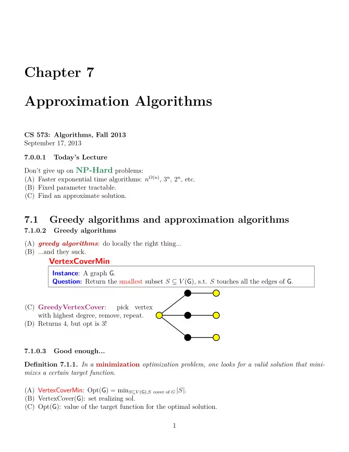VertexCoverMin Instance : A graph G . Question : Return the smallest subset S ⊆ V ( G ), s.t. S touches all the edges of G . (C) GreedyVertexCover : pick vertex with highest degree, remove, repeat. (D) Returns 4, but opt is 3! 7.1.0.3 Good enough... Definition 7.1.1. In a minimization optimization problem, one looks for a valid solution that mini- mizes a certain target function. (A) VertexCoverMin : Opt( G ) = min S ⊆ V ( G ) ,S cover of G | S | . (B) VertexCover( G ): set realizing sol. (C) Opt( G ): value of the target function for the optimal solution. 1

Definition 7.1.2. Alg is α -approximation algorithm for problem Min , achieving an approximation α ≥ 1 , if for all inputs G , we have: Alg ( G ) Opt( G ) ≤ α. 7.1.0.4 Our GreedyVertexCover Example (A) GreedyVertexCover : pick vertex with highest degree, remove, repeat. (B) Returns 4, but opt is 3! (C) Can not be better than a 4 / 3-approximation algorithm. (D) Actually it is much worse! 7.1.0.5 How bad is GreedyVertexCover? Build a bipartite graph. Let the top partite set be of size n . In the bottom set add ⌊ n/ 2 ⌋ vertices of degree 2, such that each edge goes to a different vertex above. Repeatedly add ⌊ n/i ⌋ bottom vertices of degree i , for i = 2 , . . . , n . Repeatedly add ⌊ n/i ⌋ bottom vertices of degree i , for i = 2 , . . . , n . 2

Repeatedly add ⌊ n/i ⌋ bottom vertices of degree i , for i = 2 , . . . , n . Repeatedly add ⌊ n/i ⌋ bottom vertices of degree i , for i = 2 , . . . , n . Bottom row has ∑ n i =2 ⌊ n/i ⌋ = Θ( n log n ) vertices. 7.1.0.6 How bad is GreedyVertexCover? (A) Bottom row taken by Greedy. (B) Top row was a smaller solution. Lemma 7.1.3. The algorithm GreedyVertex- Cover is Ω(log n ) approximation to the optimal solution to VertexCoverMin . See notes for details! 3

7.1.0.7 Greedy Vertex Cover Theorem 7.1.4. The greedy algorithm for VertexCover achieves Θ(log n ) approximation, where n (resp. m ) is the number of vertices (resp., edges) in the graph. Its running time is O ( mn 2 ) . Proof Lower bound follows from lemma. Upper bound follows from analysis of greedy algorithm for Set Cover , which will be done shortly. As for the running time, each iteration of the algorithm takes O ( mn ) time, and there are at most n iterations. 7.1.0.8 Two for the price of one ApproxVertexCover ( G ): S ← ∅ while E ( G ) ̸ = ∅ do uv ← any edge of G S ← S ∪ { u, v } Remove u, v from V ( G ) Remove all edges involving u or v from E ( G ) return S Theorem 7.1.5. ApproxVertexCover is a 2 -approximation algorithm for VertexCoverMin that runs in O ( n 2 ) time. Proof ... 7.2 Fixed parameter tractability, approximation, and fast ex- ponential time algorithms (to say nothing of the dog) 7.2.1 A silly brute force algorithm for vertex cover 7.2.1.1 What if the vertex cover is small? (A) G = ( V , E ) with n vertices (B) K ← Approximate VertexCoverMin up to a factor of two. (C) Any vertex cover of G is of size ≥ K/ 2. ( n K +2 ) (D) Naively compute optimal in O time. 4

7.2.1.2 Induced subgraph Definition 7.2.2. Let G = ( V , E ) be a graph. For a subset S ⊆ V , let G S be the induced subgraph over S . Definition 7.2.1. N G ( v ) : Neighborhood of v – set of vertices of G adjacent to v . v N G ( v ) 7.2.2 Exact fixed parameter tractable algorithm 7.2.2.1 Fixed parameter tractable algorithm for VertexCoverMin. Computes minimum vertex cover for the induced graph G X : 5

fpVCI ( X, β ) // β : size of VC computed so far. if X = ∅ or G X has no edges then return β e ← any edge uv of G X . ( ) β 1 = fpVCI X \ { u, v } , β + 2 ( ( ) ) β 2 = fpVCI X \ { u } ∪ N G X ( v ) , β + | N G X ( v ) | ( ( ) ) β 3 = fpVCI X \ { v } ∪ N G X ( u ) , β + | N G X ( u ) | return min( β 1 , β 2 , β 3 ). algFPVertexCover ( G =( V , E )) return fpVCI ( V , 0) 7.2.2.2 Depth of recursion Lemma 7.2.3. The algorithm algFPVertexCover returns the optimal solution to the given instance of VertexCoverMin . Proof ... u v 7.2.2.3 Depth of recursion II Lemma 7.2.4. The depth of the recursion of algFPVertexCover ( G ) is at most α , where α is the minimum size vertex cover in G . Proof : (A) When the algorithm takes both u and v - one of them in opt. Can happen at most α times. (B) Algorithm picks N G X ( v ) (i.e., β 2 ). Conceptually add v to the vertex cover being computed. (C) Do the same thing for the case of β 3 . (D) Every such call add one element of the opt to conceptual set cover. Depth of recursion is ≤ α . 6

7.2.3 Vertex Cover 7.2.3.1 Exact fixed parameter tractable algorithm Theorem 7.2.5. G : graph with n vertices. Min vertex cover of size α . Then, algFPVertexCover returns opt. vertex cover. Running time is O (3 α n 2 ) . Proof: (A) By lemma, recursion tree has depth α . (B) Rec-tree contains ≤ 2 · 3 α nodes. (C) Each node requires O ( n 2 ) work. Algorithms with running time O ( n c f ( α )), where α is some parameter that depends on the problem are fixed parameter tractable . 7.3 Traveling Salesperson Problem 7.3.0.2 TSP TSP-Min Instance : G = ( V, E ) a complete graph, and ω ( e ) a cost function on edges of G . Question : The cheapest tour that visits all the vertices of G exactly once. Solved exactly naively in ≈ n ! time. Using DP, solvable in O ( n 2 2 n ) time. 7.3.0.3 TSP Hardness Theorem 7.3.1. TSP-Min can not be approximated within any factor unless NP = P . Proof. (A) Reduction from Hamiltonian Cycle into TSP . (B) G = ( V , E ): instance of Hamiltonian cycle. (C) H : Complete graph over V .  1 uv ∈ E  ∀ u, v ∈ V w H ( uv ) = 2 otherwise .  (D) ∃ tour of price n in H ⇐ ⇒ ∃ Hamiltonian cycle in G . ⇒ TSP price at least n + 1. (E) No Hamiltonian cycle = (F) But... replace 2 by cn , for c an arbitrary number 7.3.0.4 TSP Hardness - proof continued Proof : (A) Price of all tours are either: (i) n (only if ∃ Hamiltonian cycle in G ), (ii) larger than cn + 1 (actually, ≥ cn + ( n − 1)). (B) Suppose you had a poly time c -approximation to TSP-Min . (C) Run it on H : (i) If returned value ≥ cn + 1 = ⇒ no Ham Cycle since ( cn + 1) /c > n 7

(ii) If returned value ≤ cn = ⇒ Ham Cycle since OPT ≤ cn < cn + 1 poly-time algorithm for NP-Complete problem. (D) c -approximation algorithm to TSP = ⇒ Possible only if P = NP . 7.3.1 TSP with the triangle inequality 7.3.1.1 Because it is not that bad after all. TSP △̸ = -Min Instance : G = ( V, E ) is a complete graph. There is also a cost function ω ( · ) defined over the edges of G , that complies with the triangle inequality. Question : The cheapest tour that visits all the vertices of G exactly once. triangle inequality : ω ( · ) if ∀ u, v, w ∈ V ( G ) , ω ( u, v ) ≤ ω ( u, w ) + ω ( w, v ) . ⇒ ω ( st ) ≤ ω ( σ ). Shortcutting σ : a path from s to t in G = 7.3.2 TSP with the triangle inequality 7.3.2.1 Continued... Definition 7.3.2. Cycle in G is Eulerian if it visits every edge of G exactly once. Assume you already seen the following: Lemma 7.3.3. A graph G has a cycle that visits every edge of G exactly once (i.e., an Eulerian cycle) if and only if G is connected, and all the vertices have even degree. Such a cycle can be computed in O ( n + m ) time, where n and m are the number of vertices and edges of G , respectively. 7.3.3 TSP with the triangle inequality 7.3.3.1 Continued... (A) C opt optimal TSP tour in G . ( ) (B) Observation : ω ( C opt ) ≥ weight cheapest spanning graph of G . (C) MST : cheapest spanning graph of G . ω ( C opt ) ≥ ω (MST( G )) ( n ) (D) O ( n log n + m ) = O ( n 2 ): time to compute MST . n = | V ( G ) | , m = . 2 7.3.4 TSP with the triangle inequality 7.3.4.1 2 -approximation (A) T ← MST ( G ) (B) H ← duplicate very edge of T . (C) H has an Eulerian tour. 8

(D) C : Eulerian cycle in H . (E) ω ( C ) = ω ( H ) = 2 ω ( T ) = 2 ω ( MST ( G )) ≤ 2 ω ( C opt ). (F) π : Shortcut C so visit every vertex once. (G) ω ( π ) ≤ ω ( C ) 7.3.5 TSP with the triangle inequality 7.3.5.1 2 -approximation algorithm in figures s u s u D C v C v w w (a) (b) (c) (d) Euler Tour: vuvwvsv First occurrences: vuvwvsv Shortcut String: vuwsv 7.3.6 TSP with the triangle inequality 7.3.6.1 2 -approximation - result Theorem 7.3.4. G : Instance of TSP △̸ = -Min . C opt : min cost TSP tour of G . = ⇒ Compute a tour of G of length ≤ 2 ω ( C opt ) . Running time of the algorithm is O ( n 2 ) . G : n vertices, cost function ω ( · ) on the edges that comply with the triangle inequality. 7.3.7 TSP with the triangle inequality 7.3.7.1 3 / 2 -approximation Definition 7.3.5. G = ( V, E ) , a subset M ⊆ E is a matching if no pair of edges of M share endpoints. A perfect matching is a matching that covers all the vertices of G . w : weight function on the edges. Min-weight perfect matching , is the minimum weight matching among all perfect matching, where ∑ ω ( M ) = ω ( e ) . e ∈ M 9