Chapter 4 Functional Response Theoretical Biology 2016 1 What - - PowerPoint PPT Presentation

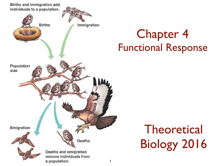
Theoretical Biology 2016 Chapter 4

Functional Response

1

What will your learn today?

To work with a saturated functional response. The humped prey nullcline. To understand the nature of oscillations. A new R0 of the predator.

Number of prey eaten per predator

f(R) h

Prey density Prey density

Prey eaten per predator

At some prey density the predator should become satiated, and/or become limited by the time to handle all the prey

3

Lotka Volterra today

LV-model has a linear functional response

(a)

R N

δ ca

K

b−d a (b)

R

δ ca

K dR dt = [b(1 − R/k) − d − aN]R and dN dt = [caR − δ]N

dR dt = [r(1 − R/K) − aN]R and dN dt = [caR − δ]N

r/a

Holling’s secretary: handling sand paper discs

y = atx and t = T − by gives y = aTx 1 + abx

Holling’s secretary: handling sand paper discs

y = atx and t = T − by gives y = aTx 1 + abx

which is a general Hill function. α=T/b is total/handling time (max number of prey) h=1/(ab) involves handling and searching times

y = aTx 1 + abx = (T/b)x 1/(ab) + x = αx h + x

Monod functional response (type II)

7

Predatory stinkbug (Podisus maculiventris) in the lab feeding

• n larvae of Mexican bean beetle.

Fitted to: y =

aTR 1+aThR where a is attack rate, T = 14 h is

total time, and Th = 0.9 h is handling time.

Linear functional response (type I)

8

Simplest type I response, y = ax + b, where b is due to other prey (mosses). Brown lemmings (Lemmus sibericus) foraging monocot in artic tundra.

From: Batzli et al., Oikos, 1981, 37: 112-116. From: Wiedenmann & O’Neil, Environ. Entomol., 1991, 20: 610-614.

40

Holling’s functional responses

9

From: Smith & Smith Elements of Ecology

Holling’s functional responses

10

From: Smith & Smith Elements of Ecology

European kestrel on Microtis vole (a), weasels on rodents in forests in Poland (b), and warblers on spruce budworm larvae (c).

Today: three formal functional responses

11

R f(R) R f(R) h R f(R) h Plotting the number of prey eaten per predator as a function

• f the prey density R.

f(R) = aR , f(R) = aR h + R and f(R) = aR2 h2 + R2

Monod predator prey model

dR dt = rR(1 − R/K) − aNR h + R dN dt = caNR h + R − dN

No R0 of the prey. For the predator we take R0 = ca/d, which is realized at large prey densities.

(instead of R0 = caK/[d(h+K)])

Nullclines

13

To sketch the nullclines we write dR/dt = 0 to find R = 0 and N = (r/a)(h + R)(1 − R/K) where the latter describes a parabola that equals zero when R = −h and R = K. For the predator nullcline we write dN/dt = 0 to find N = 0

• r

R = h ac/d − 1 which are horizontal and vertical lines in the phase space.

Nullclines

14

R N K

h R0−1

Time Population size

Predator nullcline on the right slope of parabola: Stable steady state

Nullclines

15

Predator nullcline on the left slope of parabola: Unstable steady state & stable limit cycle

R N K

h R0−1

Time

Paradox of enrichment

Increasing the prey’s carrying capacity increases the predator’s steady state level

K K K

h R0−1

Prey Predator

Paradox of enrichment: bacterial food chain

← Prey alone ← Prey with predator ← Predator

(b): The effect of nutrients on the density of prey (a): The same for prey (a: open circles) and a predator (a: closed circles). From: Kaunzinger et al. Nature 1998.

Serratia marcescens Serratia marcescens Colpidium striatium

Enrichment leads to destabilization

Steady state goes from stable spiral to unstable spiral

Hopf bifurcation

K K K

h R0−1

Prey Predator

Population cycles: periodic behavior

From Campbell

Algae zooplankton oscillations

Daphnia (blue triangles) and their edible algal prey (green squares) in four nutrient-rich systems. From: McCauley et al, Nature, 1999

Resource flows in and out by chemostat, Bacteria consume resource by a Monod function, and have an autocatalytic production of a toxin. See question 4.3 (and the GRIND files toxin.grd and toxin.txt)

20 40 60 80 1 103 106 109 1012 cell density (CFUml–1) time (h)

dR dt Z wðCKRÞKJðRÞBe; dB dt Z JðRÞBKxBT KwB; dT dt Z yBT KdT KwT:

Oscillations in continuous culture populations of Streptococcus pneumoniae: population dynamics and the evolution of clonal suicide

Omar E. Cornejo1, Daniel E. Rozen1,2, Robert M. May3 and Bruce R. Levin1,*

2009

Circadian rhythm: rodent running

Entrainment to external light From: Campbell

From: YouTube

Belousov Zhabotinsky reaction

Potassium bromate, cerium (IV) sulfate, propanedioic acid and citric acid in dilute sulfuric acid. The ratio of the cerium (IV) and cerium (III) ions oscillates, causing the color of the solution to oscillate between yellow colorless. From: YouTube

Various biological rhythms

Rhythm Period Neurons 0.01 to 10 sec Heart 1 sec Cell division 10 min to hours Circadian 24 hours Ovulation cycle 28 days Ecology years

From: YouTube

Sigmoid predator prey model

dR dt = rR(1 − R/K) − aNR2 h2 + R2

R

dR dt

K

N = small N = medium N = large

Sigmoid predator prey model

dR dt = rR(1 − R/K) − aNR2 h2 + R2

R

dR dt

K K R N K

N = y N = y