Chapter 27 Entropy, Randomness, and Information CS 573: Algorithms, - PDF document

Chapter 27 Entropy, Randomness, and Information CS 573: Algorithms, Fall 2013 December 5, 2013 27.1 Entropy 27.1.0.1 Quote “If only once - only once - no matter where, no matter before what audience - I could better the record of the great Rastelli and juggle with thirteen balls, instead of my usual twelve, I would feel that I had truly accomplished something for my country. But I am not getting any younger, and although I am still at the peak of my powers there are moments - why deny it? - when I begin to doubt - and there is a time limit on all of us.” –Romain Gary, The talent scout. 27.2 Entropy 27.2.0.2 Entropy: Definition Definition 27.2.1. The entropy in bits of a discrete random variable X is [ ] [ ] ∑ H ( X ) = − X = x lg Pr X = x . Pr x [ ] 1 Equivalently, H ( X ) = E lg . [ X ] Pr 27.2.0.3 Entropy intuition... Intuition... H ( X ) is the number of fair coin flips that one gets when getting the value of X . 27.2.0.4 Binary entropy [ ] [ ] H ( X ) = − ∑ x Pr X = x lg Pr X = x = ⇒ Definition 27.2.2. The binary entropy function H ( p ) for a random binary variable that is 1 with probability p , is H ( p ) = − p lg p − (1 − p ) lg(1 − p ) . We define H (0) = H (1) = 0 . Q: How many truly random bits are there when given the result of flipping a single coin with probability p for heads? 1

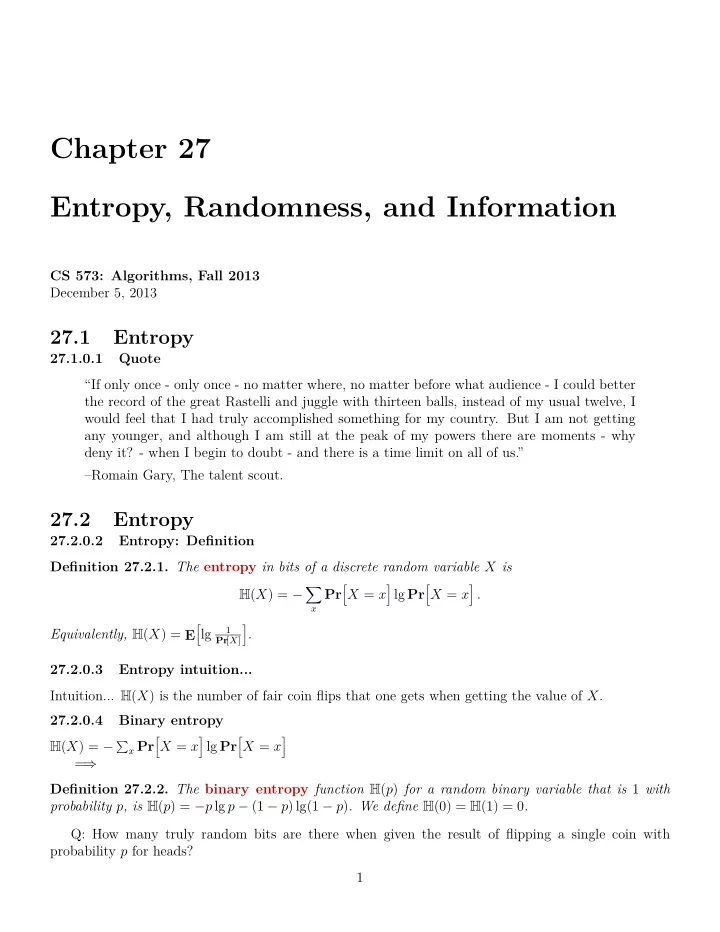
Binary entropy: H ( p ) = − p lg p − (1 − p ) lg(1 − p ) 27.2.0.5 H ( p ) = − p lg p − (1 − p ) lg(1 − p ) 1 0 . 8 0 . 6 0 . 4 0 . 2 0 0 0 . 1 0 . 2 0 . 3 0 . 4 0 . 5 0 . 6 0 . 7 0 . 8 0 . 9 1 (A) H ( p ) is a concave symmetric around 1 / 2 on the interval [0 , 1]. (B) maximum at 1 / 2. (C) H (3 / 4) ≈ 0 . 8113 and H (7 / 8) ≈ 0 . 5436. (D) = ⇒ coin that has 3 / 4 probably to be heads have higher amount of “randomness” in it than a coin that has probability 7 / 8 for heads. 27.2.0.6 And now for some unnecessary math (A) H ( p ) = − p lg p − (1 − p ) lg(1 − p ) (B) H ′ ( p ) = − lg p + lg(1 − p ) = lg 1 − p p ( ) (C) H ′′ ( p ) = p − 1 1 1 − p · = − p (1 − p ) . p 2 ⇒ H ′′ ( p ) ≤ 0, for all p ∈ (0 , 1), and the H ( · ) is concave. (D) = (E) H ′ (1 / 2) = 0 = ⇒ H (1 / 2) = 1 max of binary entropy. (F) = ⇒ balanced coin has the largest amount of randomness in it. 27.2.0.7 Squeezing good random bits out of bad random bits... Given the result of n coin flips: b 1 , . . . , b n from a faulty coin, with head with probability p , how many truly random bits can we extract? 27.2.0.8 Squeezing good random bits out of bad random bits... Question... Given the result of n coin flips: b 1 , . . . , b n from a faulty coin, with head with probability p , how many truly random bits can we extract? If believe intuition about entropy, then this number should be ≈ n H ( p ). 27.2.0.9 Back to Entropy [ ] [ ] (A) entropy of X is H ( X ) = − ∑ X = x lg Pr X = x . x Pr (B) Entropy of uniform variable.. Example 27.2.3. A random variable X that has probability 1 /n to be i , for i = 1 , . . . , n , has entropy H ( X ) = − ∑ n n lg 1 1 n = lg n . i =1 (C) Entropy is oblivious to the exact values random variable can have. (D) = ⇒ random variables over − 1 , +1 with equal probability has the same entropy (i.e., 1) as a fair coin. Lemma 27.2.4. Let X and Y be two independent random variables, and let Z be the random variable ( X, Y ) . Then H ( Z ) = H ( X ) + H ( Y ) . 2

27.2.0.10 Proof In the following, summation are over all possible values that the variables can have. By the independence of X and Y we have 1 [ ] ∑ H ( Z ) = ( X, Y ) = ( x, y ) lg Pr Pr [( X, Y ) = ( x, y )] x,y 1 [ ] [ ] ∑ = X = x Y = y lg Pr Pr Pr [ X = x ] Pr [ Y = y ] x,y 1 ∑ ∑ = Pr [ X = x ] Pr [ Y = y ] lg Pr [ X = x ] x y 1 ∑ ∑ + Pr [ X = x ] Pr [ Y = y ] lg Pr [ Y = y ] y x 27.2.0.11 Proof continued 1 ∑ ∑ H ( Z ) = Pr [ X = x ] Pr [ Y = y ] lg Pr [ X = x ] x y 1 ∑ ∑ + Pr [ X = x ] Pr [ Y = y ] lg Pr [ Y = y ] y x 1 ∑ = Pr [ X = x ] lg Pr [ X = x ] x 1 ∑ + Pr [ Y = y ] lg Pr [ Y = y ] y = H ( X ) + H ( Y ) . 27.2.0.12 Bounding the binomial coefficient using entropy ( n ) Lemma 27.2.5. Suppose that nq is integer in the range [0 , n ] . Then 2 n H ( q ) ≤ 2 n H ( q ) . n + 1 ≤ nq 27.2.0.13 Proof Holds if q = 0 or q = 1, so assume 0 < q < 1. We have ( n ) q nq (1 − q ) n − nq ≤ ( q + (1 − q )) n = 1 . nq As such, since q − nq (1 − q ) − (1 − q ) n = 2 n ( − q lg q − (1 − q ) lg(1 − q )) = 2 n H ( q ) , we have ( n ) ≤ q − nq (1 − q ) − (1 − q ) n = 2 n H ( q ) . nq 3

27.2.1 Proof continued 27.2.1.1 Other direction... ( n ) q k (1 − q ) n − k (A) µ ( k ) = k ( n ) q i (1 − q ) n − i = ∑ n (B) ∑ n i =0 µ ( i ). i =0 i ( n ) q nq (1 − q ) n − nq largest term in ∑ n (C) Claim: µ ( nq ) = k =0 µ ( k ) = 1. nq ( n ) q k (1 − q ) n − k ( ) 1 − n − k q (D) ∆ k = µ ( k ) − µ ( k + 1) = , k +1 1 − q k (E) sign of ∆ k = size of last term... ( ) ( n − k ) q (F) sign(∆ k ) = sign 1 − ( k +1)(1 − q ) ( ( k +1)(1 − q ) − ( n − k ) q ) = sign . ( k +1)(1 − q ) 27.2.1.2 Proof continued (A) ( k + 1)(1 − q ) − ( n − k ) q = k + 1 − kq − q − nq + kq = 1 + k − q − nq . (B) = ⇒ ∆ k ≥ 0 when k ≥ nq + q − 1 ∆ k < 0 otherwise. ( n ) q k (1 − q ) n − k (C) µ ( k ) = k (D) µ ( k ) < µ ( k + 1), for k < nq , and µ ( k ) ≥ µ ( k + 1) for k ≥ nq . ⇒ µ ( nq ) is the largest term in ∑ n (E) = k =0 µ ( k ) = 1. (F) µ ( nq ) larger than the average in sum. ( n ) q k (1 − q ) n − k ≥ 1 (G) = ⇒ n +1 . k ( n ) n +1 q − nq (1 − q ) − ( n − nq ) = 1 n +1 2 n H ( q ) . 1 (H) = ⇒ ≥ nq 27.2.1.3 Generalization... Corollary 27.2.6. We have: ( n ( n ) ) ≤ 2 n H ( q ) . (ii) q ∈ [1 / 2 , 1] ≤ 2 n H ( q ) . (i) q ∈ [0 , 1 / 2] ⇒ ⌊ nq ⌋ ⌈ nq ⌉ ( n ( n ) ) (iii) q ∈ [1 / 2 , 1] ⇒ 2 n H ( q ) . (iv) q ∈ [0 , 1 / 2] ⇒ 2 n H ( q ) n +1 ≤ n +1 ≤ . ⌊ nq ⌋ ⌈ nq ⌉ Proof is straightforward but tedious. 27.2.1.4 What we have... ( n ) ≈ 2 n H ( q ) . (A) Proved that nq (B) Estimate is loose. (C) Sanity check... (I) A sequence of n bits generated by coin with probability q for head. (II) By Chernoff inequality... roughly nq heads in this sequence. ( n ) ≈ 2 n H ( q ) possible sequences . (III) Generated sequence Y belongs to nq (IV) ...of similar probability. ( n ) (V) = ⇒ H ( Y ) ≈ lg = n H ( q ). nq 27.2.2 Extracting randomness 27.2.2.1 Extracting randomness... Entropy can be interpreted as the amount of unbiased random coin flips can be extracted from a random variable. 4

Definition 27.2.7. An extraction function Ext takes as input the value of a random variable X and � [ ] 1 outputs a sequence of bits y , such that Pr Ext ( X ) = y � � | y | = k = 2 k , whenever Pr [ | y | = k ] > 0 , where | y | denotes the length of y . 27.2.2.2 Extracting randomness... (A) X : uniform random integer variable out of 0 , . . . , 7. (B) Ext ( X ): binary representation of x . (C) Definition more subtle... all extracted sequence of the same length would have the same probability. (D) X : uniform random integer variable 0 , . . . , 11. (E) Ext ( x ): output the binary representation for x if 0 ≤ x ≤ 7. (F) If x is between 8 and 11? (G) Idea... Output binary representation of x − 8 as a two bit number. (H) A valid extractor... � [ ] = 1 � Pr Ext ( X ) = 00 � | Ext ( X ) | = 2 4 , 27.2.2.3 Technical lemma The following is obvious, but we provide a proof anyway. Lemma 27.2.8. Let x/y be a faction, such that x/y < 1 . Then, for any i , we have x/y < ( x + i ) / ( y + i ) . Proof : We need to prove that x ( y + i ) − ( x + i ) y < 0. The left size is equal to i ( x − y ), but since y > x (as x/y < 1), this quantity is negative, as required. 27.2.2.4 A uniform variable extractor... Theorem 27.2.9. Suppose that the value of a random variable X is chosen uniformly at random from the integers { 0 , . . . , m − 1 } . Then there is an extraction function for X that outputs on average at least ⌊ lg m ⌋ − 1 = ⌊ H ( X ) ⌋ − 1 independent and unbiased bits. 27.2.2.5 Proof (A) m : A sum of unique powers of 2, namely m = ∑ i a i 2 i , where a i ∈ { 0 , 1 } . 0 1 2 3 4 5 6 7 8 9 10 12 14 0 1 2 3 4 5 6 7 8 9 10 12 14 (B) Example: 11 13 11 13 (C) decomposed { 0 , . . . , m − 1 } into disjoint union of blocks sizes are powers of 2. (D) If x is in block 2 k , output its relative location in the block in binary representation. 0 1 2 3 0 1 2 3 4 5 6 7 8 9 10 12 14 (E) Example: x = 10: 11 13 then falls into block 2 2 ... x relative location is 2. Output 2 written using two bits, Output: “10”. 5