Chapter 25: All Pairs Shortest Paths. Context . 1. Throughout the - PDF document

Chapter 25: All Pairs Shortest Paths. Context . 1. Throughout the chapter, we assume that our input graphs have no negative cycles. 2. [ G = ( V, E ) , w : E → R ] is a weighted, directed graph with adjacency matrix [ w ij ]. Wolog, vertices are 1 , 2 , . . . , V .  0 , i = j  w ij = ∞ , i � = j and ( i, j ) �∈ E finite , i � = j and ( i, j ) ∈ E.  Note : Output is already O ( V 2 ), because for every vertex pair ( u, v ), the algo- rithm must report the weight of the shortest (weight) path from u to v . Since the output requires O ( V 2 ) work, there is no significant increase in using an O ( V 2 ) input scheme. 3. The output consists of two matrices: ∆ = δ ij = the weight of the shortest path i � j � null , if i = j or there is no path i � j Π = π ij = predecessor of j on a shortest i � j, otherwise . 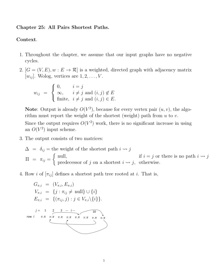4. Row i of [ π ij ] defines a shortest path tree rooted at i . That is, G π,i = ( V π,i , E π,i ) V π,i = { j : π ij � = null } ∪ { i } E π,i = { ( π ij , j ) : j ∈ V π,i \{ i }} . 1

5. Can recover a shortest path i � j with Print-Shortest-Path(Π , i, j ) { if ( i = j ) print i ; else if ( π ij = null) print(“no shortest path from i to j ”); else { Print-Shortest-Path(Π , i, π ij ); print j } } Obvious approaches. 1. If negative edges exist (but no negative cycles), we can run multiple Bellman- Ford Single-Source-Shortest-Paths, once for each v ∈ V as the Bellman-Ford source node. Since Bellman-Ford is O ( V E ), this approach is O ( V 2 E ), which is O ( V 4 ) for dense graphs ( E = Ω( V 2 )). 2. If there are no negative edges, we can run multiple Dijkstra’s, one for each v ∈ V as the Dijkstra source node. Since Dijkstra is O ( E lg V ), this approach is O ( V E lg V ), which is O ( V 3 lg V ) for dense graphs ( E = Ω( V 2 )). Improvements in this chapter, all of which work in the presence of negative edges, provided there are no negative cycles. 1. Via DP (Dynamic Programming), we can obtain Θ( V 3 lg V ). 2. Via Warshall’s Algorithm, we can obtain Θ( V 3 ). 3. Johnson’s Algorithm delivers O ( V 2 lg V + V E ). (Donald B. Johnson, 1977) This approach is better for sparse graphs, specifically for E = O ( V lg V ), we break the V 3 level with O ( V 2 lg V ). 2

The DP Algorithm . Let V = { 1 , 2 , . . . , n } , and let δ ij be the weight of the shortest-weight path from i to j . Suppose p : i � j is a shortest path from i to j containing at most m edges. As there are no negative cycles, m is finite. Let k be the predecessor of j on this path. That is, p : i � k → j . Then p ′ : i � k is a shortest path from i to k by the optimal substructure property. Moreover, the length of p ′ is at most m − 1 edges. Let δ ( m ) denote the minimum weight of any path from i to j with at most m edges. ij We have � 0 , i = j δ (0) = ij ∞ , i � = j, the lower result because, if i � = j , the set of paths from i to j containing at most zero edges is the empty set. Recall that the minimum over a set of numbers is the largest number that is less than or equal to every member of the set For m ≥ 1, � �� � � � δ ( m ) δ ( m − 1) δ ( m − 1) δ ( m − 1) = min , min + w kj = min + w kj . ( ∗ ) ij ij ik ik 1 ≤ k ≤ n 1 ≤ k ≤ n The last reduction follows because w jj = 0 for all j : � � δ ( m − 1) k = j = δ ( m − 1) + w jj = δ ( m − 1) + w kj . � ik ij ij � Now, in the absence of negative cycles, a shortest-weight path from i to j can contains at most n − 1 edges. That is δ ij = δ ( n − 1) = δ ( n ) ij = δ ( n +1) = . . . . ij ij 3

We envision a three-dimensional storage matrix, consisting of planes 0 , 1 , . . . , n − 1. In each plane, say k , is an n × n matrix of δ ( k ) values. Envision i = 1 , 2 , . . . , n as ij the row index and j = 1 , 2 , . . . , n as the column index in each plane. Recall that we are computing δ ( m ) in plane m from the row δ ( m − 1) in plane m − 1. ij i,⋆ Plane 0 is particularly easy to establish since � 0 , i = j δ (0) = ij ∞ , i � = j. Each subsequent plane fills each of n 2 cells by choosing the minimum over n values derived from the previous plane. This procedure then requires O ( n 3 ) time per plane . As we need n planes to reach the desired minimal paths lengths in δ ( n − 1) , ij we can accomplish the entire computation in O ( n 4 ) time. But, Bellman-Ford repeated V times is more straightforward, and it also runs in O ( n 4 ) time, even for dense graphs ( E = Ω( V 2 )). 4

// Θ( n 3 ) Extend-Shortest-Paths(∆ = [ δ ij ] , W = [ w ij ]) { n = row count of ∆; ∆ ′ = [ δ ′ ij ] = new n × n matrix; for i = 1 to n for j = 1 to n { δ ′ ij = ∞ ; for k = 1 to n δ ′ ij = min { δ ′ ij , δ ik + w kj } ; } return ∆ ′ ; } Slow-All-Pairs-Shortest-Paths( W = [ w ij ]) { // DP implementation n = row count of W ; ∆ = [ δ ij ] = new n × n matrix; for i = 1 to n { for j = 1 to n δ ij = ∞ ; δ ii = 0; } // Θ( n 4 ) for k = 1 to n − 1 { ∆ out = Extend-Shortest-Paths(∆ , W ); ∆ = ∆ out ; } return ∆ out ; } 5

Some helpful observations: (a) The passage from plane 0 to plane 1 is particularly easy. � ∞ , k � = i δ (0) = ik 0 , k = i � ∞ , k � = i δ (0) ik + w kj = w ij , k = i. � � δ (1) δ (0) = min ik + w kj = min {∞ , ∞ , . . . , ∞ , w ij , ∞ , . . . , ∞} = w ij . ij 1 ≤ k ≤ n Plane 1 is the input weight matrix . (b) Moreover, we can modify the initial recursion argument as follows. If, for even m , p : i � j is a shortest path of at most m edges, then we can express the path as p : i � k � j , for some intermediate vertex k , such that each of i � k and k � j contains at most m/ 2 edges. Then � �� � � � δ ( m ) δ ( m/ 2) δ ( m/ 2) + δ ( m/ 2) δ ( m/ 2) + δ ( m/ 2) = min , min = min , ij ij ik kj ik kj 1 ≤ k ≤ n 1 ≤ k ≤ n again since δ ( m/ 2) + δ ( m/ 2) = δ ( m/ 2) when k = j . ik kj ij Recall that δ whatever = 0 can not be improved in the absence of negative cycles. jj (c) Note similarity to previous recursion: � � � � δ ( m ) δ ( m − 1) δ ( m − 1) + δ (1) = min + w kj = min . ij ik ik kj 1 ≤ k ≤ n 1 ≤ k ≤ n So, Extend-Shortest-Paths(∆ = [ δ ij ] , W = [ w ij ]) can be used as Extend-Shortest-Paths(∆ ( m/ 2) , ∆ ( m/ 2) ) ij ij 6

We can now compute as follows, ∆ (1) = [ δ (1) ij ] = [ w ij ] = W ∆ (2) = [ δ (2) ij ] = Extend-Shortest-Paths(∆ (1) , ∆ (1) ) ∆ (4) = [ δ (4) ij ] = Extend-Shortest-Paths(∆ (2) , ∆ (2) ) . . . . . . Since [ δ ( k ) ij ] = [ δ ( n − 1) ] for all k ≥ n − 1, this computation will stabilize after at most ij ⌈ lg n ⌉ iterations. Fast-All-Pairs-Shortest-Paths( W = [ w ij ]) { n = row count of W ; ∆ = W ; m = 1; while m < n − 1 { ∆ = Extend-Shortest-Paths(∆ , ∆); m = 2 m ; } return ∆; } This DP computation uses lg n passes through Extend-Shortest-Paths, which is a Θ( n 3 ) algorithm. Therefore the Fast-All-Pairs-Shortest-Paths algorithm is Θ( n 3 lg n ). Consequently, this algorithm 1. beats the Θ( n 4 ) required by multiple passes through the Bellman-Ford algo- rithm, 2. ties the Θ( n 3 lg n ) required by multiple passes through the Dijkstra algorithm (which is not available is the graph contains negative edges), 3. and accommodates negative edges (although not negative cycles). 7

The Floyd-Warshall Algorithm also accommodates negative edges, although the input graph must be free of negative cycles. Let G = ( V, E ), where V = { 1 , 2 , . . . , n } . Define δ ( k ) to be the weight of the shortest path p : i � j with all intermediate ij vertices constrained to lie in the set { 1 , 2 , . . . , k } . We proceed via induction from the basis δ (0) = w ij , which reflects the constraint ij that there be no intermediate vertices. The induction step is then � � δ ( k ) δ ( k − 1) , δ ( k − 1) + d ( k − 1) = min , ij ij ik kj reflecting the fact that the shortest path with all of { 1 , 2 , . . . , k } available as inter- mediates is either (a) a path that does not use vertex k as an intermediary, or (b) a path that does use k . // Θ( n 3 ) Preliminary-Floyd-Warshall( W = [ w ij ]) { n = row count of W ; ∆ = [ δ ij ] = W ; ∆ ′ = [ δ ′ ij ] = new n × n matrix; for k = 1 to n { for i = 1 to n for j = 1 to n δ ′ ij = min { δ ij , δ ik + δ kj } ; ∆ = ∆ ′ ; } return ∆ ′ ; } Thus Floyd-Warshall, a simple data-structures algorithm, beats our best dynamic- programming algorithm: Θ( n 3 ) against Θ( n 3 lg n ). We now further develop Floyd- Warshall to capture the shortest paths themselves. 8