
SLIDE 1
1
Chapter 2 1 2.1: Inferences about 1 Test of interest throughout - - PowerPoint PPT Presentation
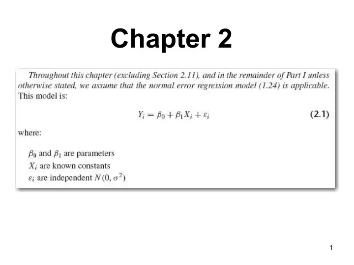
Chapter 2 1 2.1: Inferences about 1 Test of interest throughout regression: Need sampling distribution of the estimator b 1 . Idea: If b 1 can be written as a linear combination of the responses (which are independent and normally
1
2
Test of interest throughout regression: Need sampling distribution of the estimator b1. Idea: If b1 can be written as a linear combination of the responses (which are independent and normally distributed), then from A.40, we will now have the probability (sampling) distribution of b1!
3
4
Fun Fact 1. Fun Fact 2. Fun Fact 3.
5
= ?
6
7
1 2 3 4 0.0 0.1 0.2 0.3 0.4
t f(t)
8
9
10
From the sampling distribution of b1: Rearranging inside the brackets: Result:
11
Step 1: Null and alternative hypotheses: Step 2: Test statistic: Step 3: Critical Region (or see p-value):
12
S = sqrt (2384) = 48.82 Var(b1) = sqrt (2384/19800) = 0.3470 t = 3.57 / 0.3470 = 10.29 = sqrt (105.8757)
Note that 19800 = Var(X) times 24
13
14
15
Point estimate for the mean at X = Xh: For the interval estimate for the mean at X = Xh, we require the sampling distribution of Yh: ^
16
^ Yh is b0 + b1 Xh ; the b0 term is y-bar – b1 x-bar ^
17
18
19
20
Mean: Variance: Estimated Variance: Result:
21
Estimated variance of prediction: So:
22
23
We will use Yh, and our prediction error will be: pred = Yh(new) - Yh The variance of our prediction error is: Estimated by: ^ ^
24
where:
25
CH01PR19
26
27
And do all of the other Xh-points while you’re at it….
28
29
30 Y hours = 62.365859 + 3.570202*X lot size RSquare RSquare Adj Root Mean Square Error Mean of Response Observations (or Sum Wgts) 0.821533 0.813774 48.82331 312.28 25
Summary of Fit
Model Error
Source 1 23 24 DF 252377.58 54825.46 307203.04 Sum of Squares 252378 2384 Mean Square 105.8757 F Ratio <.0001* Prob > F
Analysis of Variance
Intercept X lot size Term 62.365859 3.570202 Estimate 26.17743 0.346972 Std Error 2.38 10.29 t Ratio 0.0259* <.0001* Prob>|t|
Parameter Estimates
S = sqrt (2384) = 48.82
(2384/19800) = 0.3470 t = 3.57 / 0.3470 = 10.29 = sqrt (105.8757)
Note that 19800 = Var(X) times 24
31
32
33
34
Unexplained variation before reg. Unexplained variation after reg. So what variation was explained by regression? SSR = SSTO - SSE Amazing fact:
35
But: = ? So:
36
37
38
Test Statistic: Decision Rule:
39
See text page 71. t is a Normal/sqrt(Chi-sq) so if you square t you get ______
40
F* = Critical value at .05 level:
GPA = 2.1140493 + 0.0388271*ACT RSquare RSquare Adj Root Mean Square Error Mean of Response Observations (or Sum Wgts) 0.07262 0.064761 0.623125 3.07405 120
Summary of Fit
Model Error
Source 1 118 119 DF 3.587846 45.817608 49.405454 Sum of Squares 3.58785 0.38828 Mean Square 9.2402 F Ratio 0.0029* Prob > F
Analysis of Variance
Intercept ACT Term 2.1140493 0.0388271 Estimate 0.320895 0.012773 Std Error 6.59 3.04 t Ratio <.0001* 0.0029* Prob>|t|
Parameter Estimates Linear Fit
41
Compares any “full” and “reduced” models and answers the question: Do the additional terms in the full model explain significant additional variation? (Are they needed?) Examples: Full Model Reduced Model
42
How much additional variation is explained by the full model? Result: Amazingly general test H0: Reduced model is true (R) Ha: Full model is true (F)
43
corresponding SSE(F) SSE Reduced model: Yi = β0 + εi (model under H0) corresponding SSE(R) SSTO Test statistic is F = MSR/MSE (see pages 72-73)
44
R2: Coefficient of determination Variation explained by the regression is: Total variation is: SSTO What fraction of total variation was explained by the regression? R2 = SSR/SSTO = 1 - SSE/SSTO (Rsquare) (Over-used, over-rated, possibly misleading statistic!) do not confuse with causation. As a screening tool in model selection, it is helpful.
45
46
34.4509 47.0473 32.1399 47.1475 8.9460 10.5759 35.0287 47.0223 34.4509 47.0473 12.5144 18.5112 32.1399 47.1475 8.9460 10.5759 35.0287 47.0223 12.5144 18.5112 Y1 Y2 Y3 Y4 X
R2?
47
S = 0.8194 R-Sq = 97.7% R-Sq(adj) = 97.6% S = 4.097 R-Sq = 63.4% R-Sq(adj) = 62.6% S = 0.8194 R-Sq = 0.1% R-Sq(adj) = 0.0% S = 0 R-Sq = 100.0% R-Sq(adj) = 100.0%
48
34.4509 47.0473 32.1399 47.1475 8.9460 10.5759 35.0287 47.0223 34.4509 47.0473 12.5144 18.5112 32.1399 47.1475 8.9460 10.5759 35.0287 47.0223 12.5144 18.5112 Y1 Y2 Y3 Y4 X
R2 ?
49
10 15 20
100 200 300 400 500 600 700
X Y5
Y5 = -634.823 + 53.5260 X S = 45.7285 R-Sq = 90.6 % R-Sq(adj) = 90.4 %
Regression Plot
10 15 20 32 33 34 35 36 37 38X1 Y6
50
(Not necessarily!) Example 1: GPA data! Example 2: Wrong model:
15 20 25 30 1 2 3 4ACT GPA
GPA = 1.40765 + 0.0635624 ACT S = 0.567359 R-Sq = 14.1 % R-Sq(adj) = 13.5 %Regression Plot
10 15 20 10 20 30 40 50X Y7
Y7 = 21.2853 - 0.294808 X S = 9.14570 R-Sq = 0.7 % R-Sq(adj) = 0.0 %Regression Plot
51
(Not necessarily!) Example 3: Low R2 may result from truncation
10 15 20 25 35 45 55
X Y2
52
where the sign is given by the sign of b1
53
54
55
56
57
58
conditional dists. are
be applied (Fisher’s z transformation).
59
60
61
62
63
64
65
66
67
68
69
70
71
72
73