
Chapter 19 Linear Programming II
NEW CS 473: Theory II, Fall 2015 October 29, 2015
19.1 The Simplex Algorithm in Detail
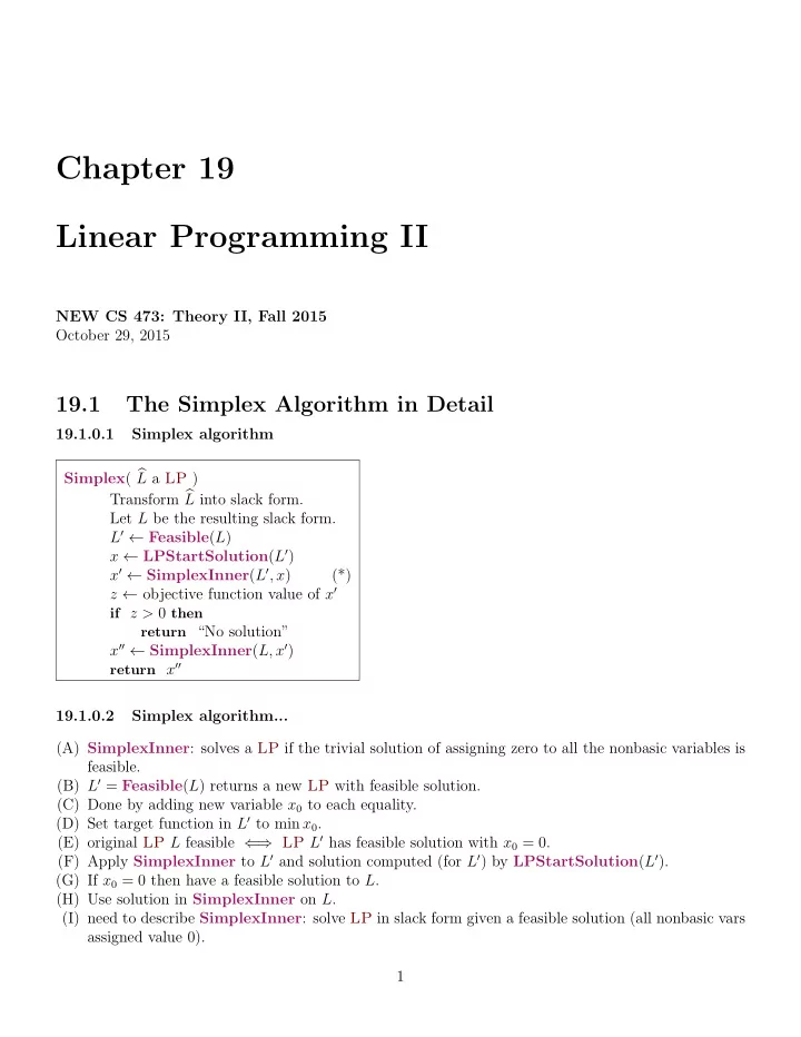
19.1.0.1 Simplex algorithm Simplex( L a LP ) Transform L into slack form. Let L be the resulting slack form. L′ ← Feasible(L) x ← LPStartSolution(L′) x′ ← SimplexInner(L′, x) (*) z ← objective function value of x′
if z > 0 then return “No solution”
x′′ ← SimplexInner(L, x′)
return x′′
19.1.0.2 Simplex algorithm... (A) SimplexInner: solves a LP if the trivial solution of assigning zero to all the nonbasic variables is feasible. (B) L′ = Feasible(L) returns a new LP with feasible solution. (C) Done by adding new variable x0 to each equality. (D) Set target function in L′ to min x0. (E) original LP L feasible ⇐ ⇒ LP L′ has feasible solution with x0 = 0. (F) Apply SimplexInner to L′ and solution computed (for L′) by LPStartSolution(L′). (G) If x0 = 0 then have a feasible solution to L. (H) Use solution in SimplexInner on L. (I) need to describe SimplexInner: solve LP in slack form given a feasible solution (all nonbasic vars assigned value 0). 1