[PDF] - Chapter 1: The integers and Obviously, this result could not be true PDF Document

SLIDE 1

F18PA2 Pure Mathematics A Number Theory & Geometry

Chapter 1: The integers and divisibility

February 19, 2016

1 / 347

The integers

We will use the set of integers: Z = {. . . , −3, −2, −1, 0, 1, 2, 3, 4, . . . } and the non-negative integers; N0 = {0, 1, 2, 3, 4, . . . } the positive integers N = {1, 2, 3, 4, . . . }

Note. Some people use the notation N for the set

{0, 1, 2, 3, 4, . . . } and some people use it for the set {1, 2, 3, 4, . . . }. To avoid this ambiguity we will use the above definitions, but we will usually avoid this notation and use the terminology ‘non-negative’ and ‘positive’ integers as defined above.

2 / 347

The integers

The set of integers Z comes equipped with:

◮ basic rules for arithmetic using addition and multiplication; ◮ ordering relation with its rules; ◮ key extra property: the well-ordering of the positive integers.

3 / 347

The relation

◮ we will use the order notation , , <, > ◮ we write, for example, a b if the integer a is less than or

equal to the integer b, so: −3 2, and 0 2 and 2 2. Note that a b allows for the possibility that a and b are equal, whereas a < b asserts that a is strictly less than and definitely not equal to b.

◮ any negative number is less than or equal to any positive

number: so −10 000 000 < 1.

◮ for every pair of integers a, b either a b or b a (or both). ◮ if a b and b a then a = b.

It is impossible for a < b and b < a to both be true.

4 / 347

The well-ordering axiom

The following well-ordering property holds in N: Theorem 1 If S is a non-empty set of positive integers then it contains an integer m such that m a for all a ∈ S. Remarks 2 In other words, any non-empty set of positive integers S contains a smallest element. Obviously, this result could not be true for an empty set, but when using the well-ordering axiom we have to remember to check that the sets we are applying it to are in fact non-empty. This harmless assertion turns out to be the principle that underlies much of our work with N and Z. Note. The well-ordering property does not hold in the set of rational numbers Q. E.g. the set {q ∈ Q : q > 0} does not have a smallest element.

5 / 347

Divisibility

Let a and b be integers. We say that b is a multiple of a, and write a|b, if there exists an integer q such that aq = b. Note that q = b/a. If b is not a multiple of a we write a | b. Equivalently, we say that a is a divisor, or a factor, of b, or that a divides b, We say that a is a proper divisor of b if 1 a < b. Be careful to distinguish a|b (statement ‘a divides b’) from a division such as a/b (the number ‘a divided by b’). E.g. 4|8 (8/4 = 2), 4 | 9 (9/4 = 2.25).

6 / 347

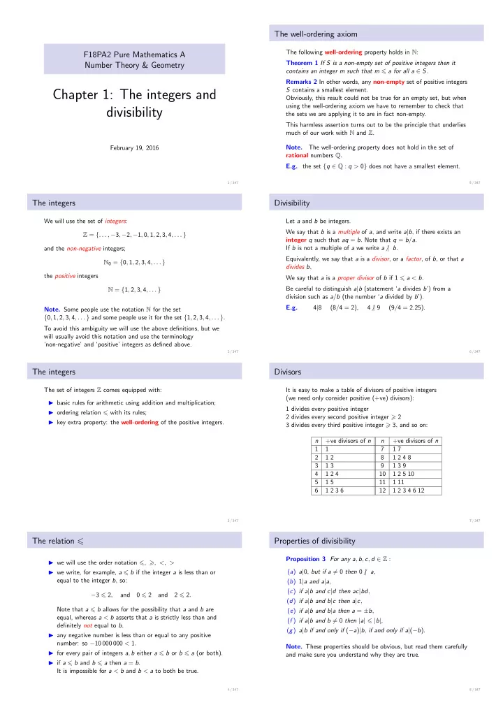
Divisors

It is easy to make a table of divisors of positive integers (we need only consider positive (+ve) divisors): 1 divides every positive integer 2 divides every second positive integer 2 3 divides every third positive integer 3, and so on: n +ve divisors of n n +ve divisors of n 1 1 7 1 7 2 1 2 8 1 2 4 8 3 1 3 9 1 3 9 4 1 2 4 10 1 2 5 10 5 1 5 11 1 11 6 1 2 3 6 12 1 2 3 4 6 12

7 / 347

Properties of divisibility

Note. These properties should be obvious, but read them carefully

and make sure you understand why they are true.

8 / 347

SLIDE 2

Some interesting functions

For a positive integer n we define the functions:

◮ τ(n) is the number of positive divisors of n (incl 1 and n), ◮ σ(n) is the sum of the positive divisors of n (incl 1 and n)

= n + the sum of the proper divisors of n. n +ve divisors τ(n) σ(n) n +ve divisors τ(n) σ(n) 1 1 1 1 7 1 7 2 8 2 1 2 2 3 8 1 2 4 8 4 15 3 1 3 2 4 9 1 3 9 3 13 4 1 2 4 3 7 10 1 2 5 10 4 18 5 1 5 2 6 11 1 11 2 12 6 1 2 3 6 4 12 12 1 2 3 4 6 12 6 28

9 / 347

A first look at prime numbers

An integer p > 1 is a prime number if its only divisors are 1 and p. By definition, the number 1 is not a prime number. We see that, for a positive integer n, n is prime ⇐ ⇒ τ(n) = 2 ⇐ ⇒ σ(n) = n + 1. The first few primes are 2, 3, 5, 7, 11, 13, 17, 19, 23, 29, 31, 37, 41, 43, 47, 53, 59, 61, 67, 71, 73, 79, 83, 89, 97, . . . and we shall see later that the list of primes goes on forever.

10 / 347

Some dull functions

For a positive integer n we also define the functions:

◮ 1

1(n) = 1 for all n,

◮ ε(1) = 1 and ε(n) = 0 if n > 1, ◮ id(n) = n for all n.

These functions seem trivial, but they give us a convenient notation for various operations.

11 / 347

Summing over divisors

Given a function f defined on N, we obtain another function F by defining F(n) =

d|n

f (d), n ∈ N. That is, the value of F at an integer n is the sum of the values of f at all the divisors d of n (this is the meaning of the d|n term below the summation sign Σ in the above formula). So, F(1) = f (1) F(2) = f (1) + f (2) F(3) = f (1) + f (3) F(4) = f (1) + f (2) + f (4) . . . F(12) = f (1) + f (2) + f (3) + f (4) + f (6) + f (12) . . .

12 / 347

Summing over divisors

Note. We get the same values in the sum for F if we write

F(n) =

d|n

f (d) =

d|n

f (n/d). We call this the usual trick for summing over divisors (we use this several times below, so make sure you understand it). F(12) =

d|12 f (d) = f (1) + f (2) + f (3) + f (4) + f (6) + f (12) =

d|12 f (n/d) = f (12) + f (6) + f (4) + f (3) + f (2) + f (1)

By the definitions of τ and σ we have: Proposition 4

◮ τ(n) =

d|n

1 1(d).

◮ σ(n) =

d|n

id(d) =

d|n

d.

13 / 347

Perfect numbers

A positive integer n is perfect if σ(n) = 2n. Or: n is perfect if it equals the sum of its proper divisors. The two smallest perfect numbers are 6 (= 1 + 2 + 3) and 28 (= 1 + 2 + 4 + 7 + 14) the third is 496. Our first observation is that these perfect numbers are all even, and this leads us to the next theorem. Theorem 5 N is even and perfect ⇐ ⇒ N = 2n−1(2n − 1), with 2n − 1 prime. The ⇐ implication was in Euclid’s Elements (circa 300 BC). The ⇒ implication was proved by Euler (1747) (but not published in his lifetime).

14 / 347

Perfect numbers

Using Theorem 5, we find the following: n 2n − 1 Is 2n − 1 prime? N = 2n−1(2n − 1) 1 1 no 1 2 3 yes 6 3 7 yes 28 4 15 no 120 5 31 yes 496 6 63 no 2016 7 127 yes 8128 The next perfect number occurs for n = 13, when N = 33 550 336.

15 / 347

Proof of Theorem 5

We will use the following key property of σ (proof later in course): if q is odd then σ(2mq) = σ(2m)σ(q). (M) (⇐) Suppose that N = 2n−1(2n − 1), with 2n − 1 prime. By (M), σ(N) = σ(2n−1)σ(2n − 1). Since the divisors of 2n−1 are 1, 2, 4, . . . , 2n−1, we have σ(2n−1) = 1 + 2 + 4 + · · · + 2n−1 = 2n − 1. (1) Since 2n − 1 is prime, we have σ(2n − 1) = 1 + (2n − 1) = 2n. Hence. σ(N) = 2n(2n − 1) = 2(2n−1(2n − 1)) = 2N, which proves the ⇐ implication. [proof of (1): S = 1 + 2 + · · · + 2n−1 = ⇒ 2S = 2 + · · · + 2n−1 + 2n, now subtract and cancel]

16 / 347

SLIDE 3

Proof of Theorem 5

(⇒) Suppose that N is even and perfect. Then N = 2n−1q, for some n 2 and odd q. Now, by (M) and (1), σ(N) = σ(2n−1)σ(q) = (2n − 1)σ(q). But N is also perfect, so σ(N) = 2N = 2nq, and combining these yields: (2n − 1)σ(q) = 2nq. σ(q) = s + q, where s is the sum of the proper divisors of q, so (2n − 1)(q + s) = 2nq = ⇒ (2n − 1)s = q. Hence:

s divides q and s < q, so s is a proper divisor of q;
s is the sum of the proper divisors of q (by definition).

This implies that s = 1, i.e., q is prime, and also q = 2n − 1 (by above, with s = 1), which proves the ⇒ implication.

17 / 347

Perfect numbers

Remarks 6

◮ Primes of the form 2n − 1 are called ‘Mersenne primes’, and

we will look at these further below.

◮ It is not known if there are any odd perfect numbers

(seriously! — this seems a trivial question, but the answer is not known).

◮ As of January 2016, 49 Mersenne primes and therefore 49

even perfect numbers are known. The largest of these is 274,207,281(274,207,281 − 1)

◮ It is not known whether there are infinitely many Mersenne

primes and perfect numbers. Remarks 7 The recent information in the remarks in these notes is usually taken from Wikipedia. It may have been updated by the time you read this

18 / 347

The division algorithm

We know that for any integers a and b we can divide a by b to find a ‘quotient’ q and a ‘remainder’ r. For example, if we divide 17 by 5 we see that 17 = 5 · 3 + 2, with quotient 3 and remainder 2. More precisely: Theorem 8 (The division algorithm) If a and b are integers with b = 0 then there exist unique integers q, r, with 0 r < |b|, such that a = bq + r. Here, q is the quotient and r is the remainder. By definition, if b > 0, the remainder r is one of the numbers 0, 1, 2, . . . , b − 1. Corollary 9 b|a ⇐ ⇒ r = 0 (i.e., b divides a iff the remainder r = 0).

19 / 347

The division algorithm

Examples. 18 = 2 · 7 + 4 26 = −3 · (−7) + 5 1234567 = 3707 · 333 + 136 10 000 000 = 8103 · 1234 + 898 9876 = (−123) · (−80) + 36. In practice, we calculate q and r by:

◮ either subtract |b| repeatedly from a until you find r, ◮ use arithmetic of rational numbers:

divide a by b to give: a/b = q + fraction (0 fraction < 1), then set the remainder r = a − bq.

20 / 347

Proof of the division algorithm

Proof. (of Theorem 8)

Existence We first prove the existence of suitable q and r, and then prove uniqueness. To avoid some trickery with modulus signs we will only deal with the case where b > 0. Suppose that b|a. Then by definition a = bq, for some integer q, so taking this integer q, together with r = 0, gives existence in this case.

21 / 347

Proof of the division algorithm

Next, suppose that b | a, and hence a = 0 and b > 1. We now define the set S = {a − bq : a − bq > 0, q ∈ Z}. The set S contains a positive integer since:

if a > 0 then a ∈ S (with q = 0);
if a < 0 then a − ba > 0 is in S (with q = a).

By the Well-Ordering Axiom, S has a smallest element, say r > 0. Hence, r = a − bq, for some integer q, and so a = bq + r.

22 / 347

Proof of the division algorithm

This argument (using the Well-Ordering Axiom) has proved the existence of suitable integers q and r. We now need to check the following properties:

r < b;
q and r are unique.

r < b Suppose that r b. If r = b then a = b(q + 1) so b divides a, which contradicts our above assumption, so in fact we must have r > b. Now, 0 < r − b = a − bq − b = a − b(q + 1) ∈ S. But r − b < r, so r − b ∈ S, since r is the smallest element of S. This contradiction shows that we must have r < b.

23 / 347

Proof of the division algorithm

q and r are unique Suppose that a = bq + r = bq′ + r′, (2) for some other integers q′, r′, with 0 r′ < b. We want to show that q = q′ and r = r′. Firstly, it is clear from (2) that if q = q′ then we must have r = r′. Suppose that q > q′ (a similar argument works for q < q′). Then by (2), a = bq + r = bq′ + r′ = ⇒ r′ − r = b(q − q′) b = ⇒ r′ b + r b. But r′ < b, so this is a contradiction, so we must have q = q′. It then follows immediately that r = r′.

24 / 347

SLIDE 4

The greatest common divisor (gcd)

Let a, b be integers, with at least one of them nonzero. A greatest common divisor (gcd) of a, b is an integer d satisfying:

d > 0,
d|a and d|b,
if c ∈ N is such that c|a and c|b then c|d.

We will prove below that a gcd exists and is unique. It will be denoted by gcd(a, b). The integers a, b are coprime (or relatively prime) if gcd(a, b) = 1. E.g. gcd(15, 25) = 5, gcd(3, 7) = 1, gcd(3, 9) = 3, gcd(6, 35) = 1.

25 / 347

The greatest common divisor (gcd)

Note. (a) The gcd is also called the highest common factor (hcf), but we will not use this terminology here. (b) When a = b = 0 the concept of the gcd of a, b does not make any sense. So, whenever we write gcd(a, b), we will suppose (without always saying so) that at least one of a or b is nonzero.

26 / 347

Existence of the gcd

Two obvious questions:

◮ Do any two integers always have a gcd? ◮ Can we calculate the gcd efficiently?

Theorem 10 Let a, b be integers, with at least one of them

nonzero. Define S be the set of all positive, integer linear

combinations of a and b: S = {au + bv : au + bv > 0, u ∈ Z, v ∈ Z}. Then S is non-empty, and its smallest element d is a gcd of a and

b. Also, the gcd is unique.

27 / 347

Proof of existence of the gcd

The set S is non-empty since, if a = 0 then |a| ∈ S, otherwise |b| ∈ S, so we can define d to be its smallest element. We now need to show that d has the properties of the gcd. By definition, d > 0 (the first property) and d = ax + by, for some x, y ∈ Z. We now want to show that d divides a and b (the second property), so we start with a (the proof for b is similar). To do this, recall from Corollary 9 of the Division Algorithm that we can test for divisibility by checking that the remainder is zero. By the Division Algorithm, a = dq + r, with 0 r < d, so that r = a − dq = a − (ax + by)q = a(1 − xq) + b(yq), that is, r is a linear combination of a and b. If r > 0 then r ∈ S, but r < d which contradicts the choice of d as the smallest element of S so r = 0 and d|a. Similarly, d|b.

28 / 347

Proof of existence of the gcd

Now suppose that c is another divisor of a and b, and write a = cr and b = cs. Then for any u, v ∈ Z, au + bv = cru + csv = c(ru + sv), so c divides every element of S. In particular, c|d (the third property). Hence, d is a gcd of a and b uniqueness Suppose that d, d′ are both gcd’s of a and b. Then d|d′ and d′|d, whence d = ±d′. But d, d′ > 0, so d = d′.

29 / 347

Properties of the gcd

The definition of the gcd, together with the construction in Theorem 10, gives: Corollary 11 Let a, b, k ∈ Z with a, k > 0. (a) gcd(a, 0) = a; gcd(a, ka) = a. (b) gcd(a, b) = gcd(b, a), (c) gcd(a, b) = gcd(−a, b) = gcd(a, −b) = gcd(−a, −b). (d) gcd(ka, kb) = k gcd(a, b) (e) If d = gcd(a, b) then gcd(a/d, b/d) = 1. That is, if we divide out the gcd of a, b, then the pair of numbers that we get is coprime. (f ) gcd(a, b) can be written as an integer linear combination gcd(a, b) = au + bv 1 for some u, v ∈ Z, and is the smallest such positive integer linear combination.

30 / 347

Properties of the gcd

We will use Corollary 11 (f ) several times below. In particular, the following special case will be used often. Corollary 12 a, b are coprime ⇐ ⇒ au + bv = 1, for some u, v ∈ Z. Note. This works because 1 is the smallest possible positive, integer linear combination. This gives a convenient arithmetical criterion for coprimality.

31 / 347

Coprime integers and divisibility

32 / 347

SLIDE 5

Coprime integers and divisibility

Intuitively, these results follow from the fact that if a, b are coprime then they have no common factors (apart from 1). For instance, in part (c) some of the factors of c must divide a and the others must divide b, but none of them can divide both (since a, b have no common factors), so we can split the factors of c up into two groups and merge them into the integers r and s to give the result. However, this is all a bit vague, and to prove the results we have to make use of more precise information following from the coprimality condition (a, b) = 1. These results and remarks should make more sense after seeing Proposition 29 below. However, we use part (b) of Proposition 13 in the proof of Proposition 29 (in fact, in the proof of Lemma 26), so we need to prove parts (a) and (b) here. Since part (c) is so similar to parts (a) and (b) we also put it here.

33 / 347

Proof of Proposition 13

Since a, b are coprime it follows from Corollary 12 that 1 = au + bv, for some u, v, ∈ Z. (3) (a) a|c and b|c = ⇒ c = ar = bs, for some r, s ∈ Z, so by (3), c = acu + bcv = absu + barv = ab(su + rv). (b) a|bc = ⇒ bc = ar, for some r ∈ Z, so by (3), c = acu + bcv = acu + arv = a(cu + rv).

34 / 347

Proof of Proposition 13

(c) Existence It will be shown in Proposition 32 below that if we put r = gcd(a, c) and s = gcd(b, c) then c = rs, r|a, and s|b. Uniqueness Suppose there are other numbers r′, s′ such that: c = r′s′, r′|a, and s′|b, with at least one of r′ = r, s′ = s. Then, from these properties, and the definition of r, s as gcd’s, r′|r and s′|s, so |r′s′| < rs = c, which contradicts r′s′ = c. So r, s must be unique. Coprimality Since a, b are coprime, it is clear that any two numbers r, s satisfying r|a and s|b must be coprime, since if they had a common factor q > 1 then q would also be a common factor of a and b.

35 / 347

The Euclidean Algorithm

The above ideas date back to Euclid (300 BC) – as does the next lemma, which will give us a practical way to compute the gcd. Lemma 14 Let a, b be integers, with at least one nonzero. If a = bq + r, for some q, r ∈ Z, then gcd(a, b) = gcd(b, r). Proof. By definition, gcd(a, b)|a and gcd(a, b)|b, and since r = a − bq we also have gcd(a, b)|r. Hence, gcd(a, b) divides both b and r, so by the definition of the gcd, gcd(a, b)| gcd(b, r). Similarly, gcd(b, r)|b, gcd(b, r)|r, a = b + rq, so gcd(b, r)|a and hence gcd(b, r) divides both a and b, so gcd(b, r)| gcd(a, b). By the properties of divisibility, gcd(a, b) = ± gcd(b, r), but both these numbers are > 0, so gcd(a, b) = gcd(b, r).

36 / 347

The Euclidean Algorithm

To compute a gcd, we combine the previous lemma with the Division Algorithm. To find gcd(a, b), for any two numbers a > b > 0:

◮ write a = bq + r with 0 r < b

(Division Algorithm);

◮ gcd(a, b) = gcd(b, r)

( Lemma 14), and the numbers in the second gcd (b and r) are smaller than in the first (a and b);

◮ repeat this process until we reach a zero remainder, when the

gcd is obvious, by part (a) of Corollary 11.

37 / 347

The Euclidean Algorithm

a = bq1 + r1 with 0 < r1 < b, gcd(a, b) = gcd(b, r1) b = r1q2 + r2 with 0 < r2 < r1, gcd(b, r1) = gcd(r1, r2) r1 = r2q3 + r3 with 0 < r3 < r2, gcd(r1, r2) = gcd(r2, r3) . . . . . . rn−2 = rn−1qn + rn with 0 < rn < rn−1, gcd(rn−2, rn−1) = gcd(rn−1, rn) rn−1 = rnqn+1 + 0 with 0 = rn+1 < rn, gcd(rn−1, rn) = rn. The remainders are integers, and reduce by at least 1 at each step, so they must eventually reach zero, and the required gcd is then the final non-zero remainder rn.

38 / 347

Euclidean Algorithm in Action

Example. Find gcd(14569, 833):

14569 = 833 × 17 + 408 833 = 408 × 2 + 17 408 = 17 × 24 (+0). So gcd(14569, 833) = 17. We can condense the writing in this example by writing: gcd(14569, 833) = gcd(833, 408) = gcd(408, 17) = 17.

39 / 347

Euclidean Algorithm in Action

gcd(14569, 833) = gcd(833, 408) = gcd(408, 17) = 17. Here, at each step we construct a new bracket from the previous bracket by:

◮ shift the right entry in the previous bracket to the left ◮ insert the remainder that we get from the two numbers in the

previous bracket into the right entry of the new bracket (you can see this shifting leftwards pattern in the calculation in Example 1 above). Note. For this process to work properly you should start with the bigger number on the left of the first bracket, and at each step you should still have the bigger number on the left.

40 / 347

SLIDE 6

Euclidean Algorithm in Action

Example. Find gcd(15572, 3298):

gcd(15572, 3298) = gcd(3298, 918) = gcd(918, 544) = gcd(544, 170) = gcd(170, 34) = 34.

41 / 347

Euclidean Algorithm in Action

So far, we have used the division algorithm to construct the remainders, which leads to positive remainders. However, we note that the basis of the algorithm, Lemma 14, did not require that the remainders be positive. In fact, if we allow negative remainders we can often get much smaller (in absolute size) remainders than just using positive remainders. This can significantly reduce the number of steps required.

42 / 347

Euclidean Algorithm in Action

Example. Find gcd(312, 184):

gcd(312, 184) = gcd(184, 128) = gcd(128, 56) = gcd(56, 16) = gcd(16, 8) = 8. gcd(312, 184) = gcd(184, −56) = gcd(184, 56) = gcd(56, 16) = gcd(16, 8) = 8. Here, at the step marked in red, we have used 312 = 2 × 184 − 56, where in the first calculation we used 312 = 1 × 184 + 128. That is we have subtracted one more copy of 184 from 312, and gone down to a (smaller) negative remainder.

43 / 347

Euclidean Algorithm in Action

The red equality gcd(184, −56) = gcd(184, 56), follows from part (c) of Corollary 11. This is a trivial computation (we have just dropped the minus sign), so comparing the second calculation with the first one we see that the remainders have decreased more quickly, and we have done one less ‘nontrivial’ calculation. This may not seem much, but in a big calculation the savings this yields can add up.

44 / 347

Euclidean Algorithm runtime

It might seem like the Euclidean algorithm would take a long time to run if we started with big numbers, but in fact it is astonishingly

fast. Let’s try to quantify this.

The following lemma shows that if we allow negative remainders then at each step they don’t just go down by 1, they more than halve (this will probably become clear when you have done a few examples — you need to do these yourself, you won’t get the hang

f all this just by reading the ones I have done).

45 / 347

Euclidean Algorithm runtime

Lemma 15 If we allow negative remainders ri, i = 1, . . . , n, in the Euclidean algorithm then they can be chosen so that |ri+1| 1 2|ri|, i = 1, . . . , n.

Proof. For simplicity, suppose that we are at the ith step, that

ri > 0, and that if we choose the remainder by the division algorithm, call it r+

i+1 > 0, then r+ i+1 isn’t small enough. That is,

0 < 1 2ri < r+

i+1 < ri.

Defining r−

i+1 = r+ i+1 − ri, we see by subtracting ri from these

inequalities, that −1 2ri < r−

i+1 < 0 =

⇒ |r−

i+1| < 1

2ri, so that r−

i+1 is a negative remainder, and it is small enough.

46 / 347

Euclidean Algorithm runtime

Halving at each step is a very fast way of going to zero — let’s see what this implies for the number of steps the Euclidean algorithm takes to finish. For given a > b > 0, let N(a, b) denote the number of steps that the Euclidean algorithm takes to finish (so N(a, b) = n + 1 in the above outline of the algorithm). Lemma 16 Given any a > b > 0, if we choose the smallest remainders at each step of the algorithm (allowing negative remainders), then N(a, b) log b log 2. (4)

47 / 347

Euclidean Algorithm runtime

Remarks 17 Lemma 16 shows that the Euclidean algorithm runs amazing quickly. Cryptography routinely needs to find the gcd of pairs of numbers

f the order of 10100 or 101000, and the Euclidean algorithm can do

this in about 100, or 1000, steps. These numbers are astonishingly big — don’t be fooled by the small looking exponents 100 or 1000. Remember that a trillion is merely 1012, and the number of atoms in the universe is only about 1080.

48 / 347

SLIDE 7

Euclidean Algorithm runtime

Proof. By Lemma 15, we have

|r1| 2−1b, |r2| 2−1|r1| 2−2b, . . . |ri| 2−1|ri−1| 2−ib, . . . So if, after k steps, we have 2−kb < 1 then |rk| must be zero (since it is an integer), and so the algorithm must already have

finished. Rearranging this inequality and taking logs gives

2−kb < 1 ⇐ ⇒ 2k > b ⇐ ⇒ k log 2 > log b ⇐ ⇒ k > log b log 2.

49 / 347

Euclidean Algorithm runtime

Rearranging the last two sentences gives: if we take k > log b log 2 steps then the algorithm must already have finished, so the number of steps we actually took to finish, N(a, b), must satisfy N(a, b) log b

log 2 (it may be a lot less than that if we are

lucky).

50 / 347

The magic matrix method

For any a, b ∈ N, Corollary 11 showed that gcd(a, b) can be written as the smallest positive integer linear combination of a, b. It is often useful to know what this linear combination is, so we now investigate how to find it. One way is to ‘reverse’ the calculations in the Euclidean algorithm. For instance, we showed in Example 1 above that gcd(14569, 833) = 17, and ‘reversing’ the calculations there gives 17 = 833 − (408 × 2) = 833 − ((14569 − 833 × 17) × 2) = 833 × 35 − 14569 × 2. However, it would be nice to have a more systematic, and easy to apply, procedure than this. In fact, an extension of the Euclidean algorithm, called the magic matrix method (or sometimes Blankinship’s algorithm) does this.

51 / 347

The magic matrix method

To apply the magic matrix method we begin with the matrix a 1 b 1

,

and carry out the following row operations, aiming to obtain a zero in the first column:

◮ add an integer multiple of one row to the other row; ◮ change the sign of all the entries in a row; ◮ stop once you obtain a zero in the first column.

Now, change the sign of the row with non-zero first entry, if necessary, so that it looks like (d, u, v), with d > 0. Then gcd(a, b) = d = au + bv, which is the desired integer linear combination.

52 / 347

The magic matrix method

Note. You can stop when a zero will be obtained in the first column at the next use of a row operation, since the required information is already in the other row. Note. The basic Euclidean algorithm is a very slick way of finding gcd(a, b), so the magic matrix method is only really worthwhile if we also need to express gcd(a, b) as a linear combination of a and b (which the basic Euclidean algorithm is not so good at). A proof of why the magic matrix method works is sketched in the notes — we will simply give an example here.

53 / 347

The magic matrix method

Example. To find gcd(14569, 833):

14569 1 833 1

R1−17·R2

→ 408 1 −17 833 1

R2−2·R1

→ 408 1 −17 17 −2 35

.

Since 17 | 408 a zero will occur in the top row at the next step. Hence, from the second row: gcd(14569, 833) = 17 = −2 × 14569 + 35 × 833. Do lots of these examples yourself! We will use these methods repeatedly, and you won’t be able to do it yourself unless you practice it.

54 / 347

F18PA2 Pure Mathematics A Number Theory & Geometry

Chapter 2: Linear Diophantine Equations

55 / 347

Linear Diophantine Equations

Problem: Given integers a, b, c, find all integers x, y such that ax + by = c. (5) Note. The restriction to integers for the coefficients a, b, c and the solution (x, y) is what makes the problem (5) hard — without this restriction the problem would be trivial. Such problems were considered by Diophantus of Alexandria (c. 200–284 AD), and so are called Diophantine. There may be no solution. For example, the equation 6x + 10y = 23 has no solution since 6x + 10y is always even, and 23 is odd. By using gcd’s we can tell whether or not there is a solution.

56 / 347

SLIDE 8

Solving Diophantine Equations

If (5) has a solution: gcd(a, b) divides ax + by, so gcd(a, b) | c. If gcd(a, b) | c: say c = gcd(a, b)q for some integer q, then we can construct a solution as follows: by the Euclidean algorithm au + bv = gcd(a, b), (6) for some u, v ∈ Z, and multiplying (6) by q gives a(qu) + b(qv) = gcd(a, b)q = c, so we get the solution x0 := qu = uc gcd(a, b), y0 := qv = vc gcd(a, b). (7) Note. It is quite easy find gcd(a, b) and u, v ∈ Z, in (6), and the solution in (7) then comes from simply scaling up (6). Thus, this process gives us a practical procedure for actually finding the solution (x0, y0) in (7).

57 / 347

Solving Diophantine Equations

It turns out that if there is one solution then there are infinitely many, and we will describe them all. If (x0, y0) is a solution of (5), then we can add any solution (z1, z2)

f the equation

az1 + bz2 = 0 (8) to (x0, y0) to get another solution (x0 + z1, y0 + z2) of (5). Equation (8) always has solutions. An obvious one is (z1, z2) = (b, −a) and a slightly less obvious one is (z1, z2) =

b

gcd(a, b), − a gcd(a, b)

.

Any integer multiple t(z1, z2), t ∈ Z, of (z1, z2) is also a solution

f (8), so adding all such multiples to (x0, y0) gives us infinitely

many solutions of (5).

58 / 347

Solving Diophantine Equations

We summarize these remarks, and show that they give the full set

f solutions of (5) in the next theorem.

For the rest of this section we will use the notation

a =

a gcd(a, b),

b =

b gcd(a, b),

c =

c gcd(a, b), (9) which will simplify some of the above formulae (we only use the notation c when gcd(a, b)|c).

59 / 347

Solving Diophantine Equations

Theorem 18 (a) The equation ax + by = c has a solution ⇐ ⇒ gcd(a, b)|c. (b) If there is a solution (x0, y0), then there are infinitely many solutions (x, y), given by x = x0 + bt gcd(a, b) = x0 + bt, y = y0 − at gcd(a, b) = y0 − at, (10) for any t ∈ Z. In addition, the formula (10) gives all the solutions of (5). Note. Of course, the obvious solution to use in (10) is (x0, y0) = (u c, v c) as given in (7), where u, v come from the gcd linear combination (6). Corollary 19 If a, b are coprime (i.e., gcd(a, b) = 1) then (5) has a solution.

60 / 347

Proof

Proof. (a) We have already proved part (a) in the preceding

discussion. (b) It is easy to check, by substitution, that the formula (10) does in fact give a solution for any t ∈ Z, which proves the first statement in part (b). We now have to show that every solution arises from (10).

61 / 347

Proof (continued)

Let x′, y′ be an arbitrary solution. Then ax′ + by′ = ax0 + by0 = c, and so a(x′ − x0) + b(y′ − y0) = 0 (i.e., (x′ − x0, y′ − y0) satisfies (8)). Dividing this equation by gcd(a, b) and rearranging gives

a(x′ − x0) =

b(y0 − y′) and gcd( a, b) = 1 (by part (e) of Corollary 11). Hence, by part (b) of Proposition 13,

a divides y0 − y′, say

at = y0 − y′, and so y′ = y0 − at, as claimed. Also,

a(x′ − x0) =

a bt = ⇒ x′ = x0 + bt.

62 / 347

Solving Diophantine Equations - examples

Examples

(1) 4x + 16y = 7 has no solutions, since a = 4, b = 16, gcd(a, b) = 4, c = 7 and 4 | 7. This should be obvious at a glance, since the left hand side is even (whatever x and y are), and the right hand side is odd. (2) Find the solutions of 5x + 2y = 185.

Ans. Here, a = 5, b = 2, gcd(a, b) = 1, so Corollary 19 applies

and shows that solutions exist. To find these, note that 1 = 5−2·2 = ⇒ 185 = 185·5−185·2·2 = ⇒ (185, −370) is a solution. The other solutions are now given by x = 185 + 2t, y = −370 − 5t, t ∈ Z.

63 / 347

Solving Diophantine Equations - examples

Remarks. (a) In Ex. 2 it was easy to spot the gcd and the lin comb — in general, we would need the Euclidean algorithm to find these. (b) The linear combination is not unique. We used 1 = 5 − 2 · 2 above, but we could use 1 = (−1) · 5 + 3 · 2, to give a solution (−185, 555), and then the general solution, say, x = −185 + 2s, y = 555 − 5s, s ∈ Z. This looks quite different to what we had before, but if we put s = t + 185 it turns into the previous formula. So, the two linear combinations yield different ‘starting solutions’ (x0, y0), but the same overall infinite set of solutions. Any other linear combination would do the same.

64 / 347

SLIDE 9

The Frobenius Problem

Named after Georg Frobenius (1849-1917) and also called the Coin (or Stamp) Problem. Suppose you have an unlimited quantity of coins of values a and b.

Qu. Can you combine these coins to get any required total value?
Ans. No:

◮ if gcd(a, b) = d then any value obtained is divisible by d.

Qu. Suppose that gcd(a, b) = 1: can you do it now?
Ans. No:

◮ there are small values that you can’t get;

e.g., if a = 5 and b = 6 then gcd(a, b) = 1, but obviously you can’t get anything < 5, or you can’t get 7, say.

65 / 347

The Frobenius Problem

Theorem 20 Let a, b be coprime positive integers. Then there is a largest integer not expressible as au + bv with u, v non-negative

integers. This is the Frobenius number, g(a, b), of a and b, and

g(a, b) = ab − a − b. Example 21 If a = 5 and b = 6 then g(a, b) = 30 − 5 − 6 = 19. Hence 19 cannot be written as a non-negative integer linear combination of 5 and 6, but every integer 20 can be. The last fact is easily demonstrated by writing 20, 21, 22, 23, 24 in terms of 5 and 6, and then any other integer > 24 can be obtained from one of these by adding multiples of 5.

66 / 347

Proof

Let m 1 be an arbitrary integer. Since a, b are coprime we have ar + bs = 1, for some integers r, s, so m can be written as m = a(rm) + b(sm) = ax + by, where x = rm, y = sm, and in fact m can be expressed as m = a(x − tb) + b(y + ta), for arbitrary t ∈ Z (clearly the abt terms cancel out). This has expressed an arbitrary integer m as an integer linear combination of a and b. However, we want non-negative coefficients in the linear combination, and this will restrict the possible values of m.

67 / 347

Proof

Now, by the Division Algorithm, we can choose t = tr such that 0 x − trb b − 1 (writing x = trb + remainder), so, putting u = x − trb, v = y + tra, we conclude that any integer m 1 can be written in the form m = au + bv, with 0 u b − 1. Now suppose that m 1 is not expressible in the required form (that is, with both coefficients u, v non-negative). Then we must have m = au + bv, with 0 u b − 1 and v −1. The largest such m occurs when u = b − 1 and v = −1, giving g(a, b) = a(b − 1) − b = ab − a − b.

68 / 347

F18PA2 Pure Mathematics A Number Theory & Geometry

Chapter 2: Prime Numbers

69 / 347

Prime numbers

A prime number is an integer p 2 which has no positive divisors except itself and 1. An integer n 2 that is not prime is called composite. A proper divisor of n is an integer d that divides n, and 1 d < n. The number 1 is not a prime number. We see from the definitions that for n 1, n is prime ⇐ ⇒ τ(n) = 2 ⇐ ⇒ σ(n) = n + 1.

70 / 347

Prime numbers

Theorem 22 Any n 2 is either prime or a product of primes.

Proof. Let S be the set of integers n 2 that are neither prime

nor a product of primes (i.e., S is the set of integers n 2 that does not have the property in the theorem). We want to show that S is empty. Suppose that S = ∅. Then it has a smallest element, say m. Since m ∈ S, m is not prime, so m = ab with a, b smaller than m. Since m is the smallest element of S, neither a nor b are in S, so each is either prime or a product of primes. In either case, m = ab is a product of primes, and so m ∈ S. This contradicts the choice of m = ⇒ S = ∅ = ⇒ every integer n 2 has the property in the theorem.

71 / 347

Infinitely many primes . . .

The next result was in Book IX of ‘The Elements’, by Euclid. Theorem 23 There are infinitely many primes.

Proof. Suppose we have a finite collection of primes, say

p1, p2, · · · , pk. We will find a prime not in this list. Let nk = (p1 × p2 × · · · × pk) + 1. Either nk is prime or it is composite. If nk is prime then it is new (it is larger than the original primes). If nk is composite, let q be a prime divisor of nk (q exists by the previous theorem). Since all the primes p1, p2, · · · , pk leave remainder 1 when dividing nk, none of them can equal q, so we again get a new prime.

72 / 347

SLIDE 10

New prime number found

January 2016 A new, largest, prime number has just been found: 274,207,281 − 1 which is a Mersenne prime. In decimal notation, this has about 22.5 million digits. To date, 49 Mersenne primes are known. Since 1997, all newly found Mersenne primes have been discovered by the ’Great Internet Mersenne Prime Search’ (GIMPS), a distributed computing project on the Internet.

73 / 347

Finding prime numbers (Sieve of Eratosthenes)

Lemma 24 If n 2 is composite then it has a prime divisor p √n.

Proof. Suppose that n = ab with 1 < a b. Then a2 ab = n

and taking square roots gives a √n. This result justifies the Sieve of Eratosthenes (276-194 BC), which finds all primes p with 1 < p n:

◮ Write out all the integers from 2 to n. ◮ Cross out all the multiples of primes 2, 3, . . . up to the largest

prime less than or equal to √n.

◮ By Lemma 24, any number not crossed out must be prime.

We find there are 25 primes less than 100, 168 primes less than 1000, and 1229 primes less than 10000.

74 / 347

SLIDE 11

The Prime Number Theorem

For any integer n 2, let π(n) = the number of primes p n. Theorem 25 lim

n→∞

π(n) n/ loge(n) = 1. This was first proved in 1896 – independently, by the Belgian C.J. de la Vall´ ee-Poussin and the French mathematician J. Hadamard. There are more accurate modern versions of this theorem, with estimates for how good the approximations are.

81 / 347

The Prime Number Theorem

The rate of convergence in Theorem 25 n π(n)

n loge(n) π(n) n/ loge(n)

π(n) − n/ loge(n) 101 4 4.3 0.921 −0.3 102 25 21.7 1.151 3.3 103 168 144.7 1.161 23 104 1, 229 1,085.7 1.132 143 105 9, 592 8,685.9 1.104 906 106 78, 498 72,382.4 1.084 6, 116 . . . 1025 176 × 1021 1.018

The ratio

π(n) n/ loge(n) does tend towards 1, but the rate of

convergence is very slow!

The difference π(n) − n/ loge(n) grows and tends to ∞.

82 / 347

The Prime Number Theorem

The proportion of prime numbers below n The proportion of prime numbers below n, to n is 1 loge n = log10 e log10 n ≈ .435 log10 n, that is ≈ 43.5 log10 n% Some examples are given in the following table. n Approx proportion Actual proportion prime (%) prime (%) 102 21.7 25 103 14.5 16.8 104 10.8 12.3 . . . 10100 .435 ?? 101000 .0435 ??

83 / 347

The Prime Number Theorem

This shows that although the proportion of primes to composite numbers is decreasing, it is not decreasing very fast (when n is big, the quantity log10 n is very small compared to n).

84 / 347

The fundamental theorem of arithmetic

We have seen that every positive integer can be expressed as a product of primes ( Theorem 22). We now show that this can be done in only one way. This is called unique factorisation into primes. This uniqueness is the main reason we don’t consider 1 as a prime, since if we did the uniqueness would fail: 6 = 2 × 3 = 1 × 2 × 3 = 1 × 1 × 2 × 3 = · · ·

85 / 347

The fundamental theorem of arithmetic

To prove the uniqueness of prime factorizations we first need a lemma about divisibility by primes. Lemma 26 If a prime number p divides a product a1a2 · · · ak then p divides aj for some j.

Proof. If p|a1 we are done.

Otherwise, gcd(p, a1) = 1 and p divides a2 · · · ak (by Proposition 13 (b)). Repeat this process until we find a suitable aj (we might get to the end and find that p divides ak).

86 / 347

The fundamental theorem of arithmetic

Theorem 27 Any integer n 2 is a product of primes, and this factorization is unique (up to the order of the factors).

Proof. We have seen that n can be factorised into primes.

Now suppose that n has two different factorizations, n = p1 · · · pr = q1 · · · qs (where pi, qj are prime). Since p1|n, it follows from Lemma 26 that p1|qj, for some j, and since qj is prime and p1 = 1 we have p1 = qj. Now relabel the qj factors so that j = 1, and we then have n = p1p2 · · · pr = p1q2 · · · qs, and so p2 · · · pr = q2 · · · qs.

87 / 347

Proof

(proof continued) p2 · · · pr = q2 · · · qs. Repeating the argument we deduce that p2 = q2 (after another relabelling, if necessary), and we can continue this process until we have relabelled all the qj’s into pi’s.

88 / 347

SLIDE 12

Unique prime decomposition

If we fix an ordering for the primes in a factorization, say, increasing order, we get the following result. Theorem 28 (Unique prime decomposition) Any integer n 2 can be written uniquely as n = pα1

1 pα2 2 · · · pαk k ,

with primes p1 < p2 < · · · < pk, and each αj 1.

89 / 347

Formulae for τ, σ and the gcd

Proposition 29 (a) Let n = pα1

1 pα2 2 · · · pαk k . Then:

◮ τ(n) = (α1 + 1)(α2 + 1) · · · (αk + 1); ◮ σ(n) = pα1+1

1

− 1 p1 − 1 pα2+1

2

− 1 p2 − 1 · · · pαk+1

k

− 1 pk − 1 . (b) If m, n 2 are integers and qj, j = 1, . . . , s, are the primes

ccurring in both of the prime decompositions of m and n,

with respective powers αj and βj, then gcd(m, n) = qmin{α1,β1}

1

· · · qmin{αs,βs}

s

.

90 / 347

Formulae for τ, σ and the gcd

Proof. (a) For simplicity, let k = 2. Now, any factor of n has the

form pγ1

1 pγ2 2 , with 0 γj αj. Hence, we can list the factors as:

p0

1p0 2, p0 1p1 2, . . . , p0 1pα2 2 ,

p1

1p0 2, p1 1p1 2, . . . , p1 1pα2 2 ,

. . . pα1

1 p0 2, pα1 1 p1 2, . . . , pα1 1 pα2 2 .

We conclude that τ(n) = (1 + α1)(1 + α2) σ(n) = (p0

1 + p1 1 + · · · + pα1 1 )(p0 2 + p1 2 + · · · + pα2 2 )

= pα1+1

1

− 1 p1 − 1 pα2+1

2

− 1 p2 − 1 (using the sum of a geometric progression to get the final equality).

91 / 347

Formulae for τ, σ and the gcd

(b) Let d = qmin{α1,β1}

1

· · · qmin{αs,βs}

s

. (11) We will check that d satisfies all the conditions in the definition of the gcd(m, n), which, by Theorem 10, shows that d = gcd(m, n). Firstly, d > 0 and it is clear from the definition of d in terms of prime factors of m and n that d|m and d|n, so the first two conditions hold.

92 / 347

Formulae for τ, σ and the gcd

Now suppose that c is such that c|m, c|n. Then it follows from the uniqueness of prime factorisations (Theorem 27) that:

any prime factor q of c must be a prime factor of both m and

n, so q must be in the list q1, . . . , qs;

the number of times q occurs in the factorisation of c must

be less than the number of times it occurs in the factorisation

f either m or n.

Hence, c must have a prime factorisation of the form c = qγ1

1 · · · qγs s ,

0 γj min{αj, βj}, j = 1, . . . , s. (12) Comparing the factorisations (11) and (12), we see that c|d, so d satisfies the third condition in the definition of gcd(m, n).

93 / 347

Formulae for τ, σ and the gcd

Examples. (a) m = 11250 = 2·32·54, n = 65625 = 3·55·7, gcd(m, n) = 3·54. (b) Let m = 2529527 and n = 417146653. Trial division by small primes finds the prime decompositions m = 72 · 11 · 13 · 192 n = 73 · 112 · 19 · 232. Hence τ(n) = 4 · 3 · 2 · 3 = 72, σ(m) = 73 − 1 7 − 1 · 112 − 1 11 − 1 · 132 − 1 13 − 1 · 193 − 1 19 − 1 = 57 · 12 · 14 · 381 = 3648456, gcd(m, n) = 72 · 11 · 19 = 10241.

94 / 347

Formulae for τ, σ and the gcd

Remarks 30 We see from these examples, and Proposition 29, that we obtain gcd(m, n) from the prime factorisations of m and n by ‘pulling out’ as many joint factors of m and n as we can. Part (b) of Proposition 29 also yields the following result. Corollary 31 Integers m, n 2 are coprime ⇐ ⇒ no prime p

ccurs in both of the prime decompositions of m and n.

95 / 347

Formulae for τ, σ and the gcd

We can also use the above results to give the existence part of the proof of part (c) of Proposition 13, which we restate here in full. Proposition 32 Suppose that a, b, c ∈ N, are such that a, b are coprime and c|ab. Then there exists unique coprime positive integers r, s such that c = rs, r|a, s|b. (13) In fact, we have r = gcd(a, c) and s = gcd(b, c).

Proof. We showed previously that if numbers r, s exist for which

(13) holds, then they must be unique and coprime. Thus it suffices to show that if we set r = gcd(a, c) and s = gcd(b, c) then (13) holds.

96 / 347

SLIDE 13

Formulae for τ, σ and the gcd

Since a, b are coprime and c|ab, by Corollary 31 any prime factor p of c must be a prime factor of one of a or b, but not both. So, we can write the prime factorisations of a, b, c in the form c = r ˜

α1 1 · · · r ˜ αk k s ˜ β1 1 · · · s ˜ βl l ,

a = rα1

1 · · · rαk k P,

αi ˜ αi, i = 1, . . . , k, b = sβ1

1 · · · sβl k Q,

βi ˜ βi, j = 1, . . . , l, where P, Q contain the prime factors of a, b other than the ri’s and sj’s (which are the factors of c). Now, setting r = r ˜

α1 1 · · · r ˜ αk k ,

s = s

˜ β1 1 · · · s ˜ βl l ,

we see that (13) is satisfied.

97 / 347

Formulae for τ, σ and the gcd

The fact that r = gcd(a, c) and s = gcd(b, c) follows from Part (b) of Proposition 29 together with the above prime factorisations of a, b, c. Remarks 33 The existence result in Proposition 32 could have been proved in the gcd section, using the methods developed there, and this would have seemed more logical. However, the method used here seems clearer and better illustrates the relationship between the gcd and prime factorisation.

98 / 347

The least common multiple

Given two integers a and b, if a|c and b|c then we say that c is a common multiple of a and b. The smallest common multiple of a and b is called the least common multiple of a and b and will be denoted by lcm(a, b). We do not need a new algorithm to calculate the least common multiple, we can use Euclid’s algorithm for the gcd, together with the following result. Proposition 34 Let a, b be positive integers. Then gcd(a, b) · lcm(a, b) = ab.

99 / 347

The least common multiple

Proof. We write a, b in the form

a = pα1

1 pα2 2 . . . pαk k

and b = pβ1

1 pβ2 2 . . . pβk k ,

where each pi is prime and αi 0, βi 0, αi + βi 1 [see the notes for why we can do this]. Then gcd(a, b) = pmin(α1,β1)

1

× · · · × pmin(αk,βk)

k

, lcm(a, b) = pmax(α1,β1)

1

× · · · × pmax(αk,βk)

k

, and hence, gcd(a, b) · lcm(a, b) = pmin(α1,β1)+max(α1,β1)

1

× . . . × pmin(αk,βk)+max(αk,βk)

k

= pα1+β1

1

× · · · × pαk+βk

k

= ab

100 / 347

Special types of primes: Mersenne primes

A Mersenne prime is a prime of the form 2k − 1 Mersenne primes are named after Marin Mersenne (1588-1648). Lemma 35 If p = ak − 1 is prime then a = 2 and k must be prime.

Proof. Since

ak − 1 = (a − 1)(ak−1 + ak−2 + · · · + 1), we see that a − 1 divides ak − 1, so, ak − 1 is prime = ⇒ a − 1 = 1 = ⇒ a = 2. Now, if k = rs is composite then 2k − 1 = 2rs − 1 = (2r − 1)(2r(s−1) + 2r(s−2) + · · · + 2r + 1), and so 2k − 1 is composite.

101 / 347

Special types of primes: Mersenne primes

This lemma does not say that: k is prime = ⇒ 2k − 1 is prime. The following is a counterexample: 211 − 1 = 2047 = 23 × 89.

102 / 347

Special types of primes: Mersenne primes

The search for big primes looks for Mersenne primes: this is coordinated by the Great Internet Mersenne Prime Search, at www.mersenne.org. As of January 2016, just 49 Mersenne primes are known, and the current largest is 274,207,281 − 1 which has about 22.5 million digits [look for yourself to see if this has been beaten yet]. The reason people look for big Mersenne primes is that there are some special, extremely efficient, tests to decide if a number of the Mersenne type is prime which do not apply to general numbers. Hence, much bigger Mersenne type numbers can be tested than is the case for general numbers. Even these test take a long time to run!

◮ Are there infinitely many Mersenne primes?

It isn’t known.

103 / 347

Special types of primes: Fermat primes

A Fermat prime is a prime of the form 2k + 1. Fermat primes are named after Pierre de Fermat (1601-1665) (he also has a more famous ‘Fermat’s last theorem’ named after him, see below). Lemma 36 If p = 2k + 1 is prime then k must be a power of 2. The proof of this is not hard, but it relies on congruences, which we will discuss in Chapter 4, so we will skip this proof. The lemma does not say that: k is a power of 2 = ⇒ 2k + 1 is a prime. Writing Fn = 22n + 1, n 0, only five Fermat primes are known: F0 = 3, F1 = 5, F2 = 17, F3 = 257, F4 = 65537.

◮ Are there infinitely many Fermat primes?

104 / 347

SLIDE 14

Some related questions

Over the years people have considered many, many questions about primes. The following is a small selection. The first one is true; ; whether the others are true is not yet known (or is it?).

◮ Dirichlet’s Theorem. If gcd(a, d) = 1 the arithmetic

progression a, a + d, a + 2d, a + 3d, . . . contains infinitely many primes.

◮ (Twin primes) Are there infinitely many primes p such that

p + 2 is also prime? E.g., 3,5, 5,7, 11,13, 17,19.

105 / 347

Update on twin primes

From Wikipedia: On April 17, 2013, Yitang Zhang announced a proof that there are infinitely many pairs of consecutive primes with gaps at most 70 million. This proof is the first to establish the existence of a finite bound for prime gaps, resolving a weak form of the twin prime conjecture. The twin prime conjecture asserts that there are infinitely many pairs of consecutive primes with a gap of size 2. Zhang’s paper was accepted by Annals of Mathematics in early May 2013.

106 / 347

Some related questions

◮ (Goldbach’s conjecture) Every even integer m > 2 can be

expressed as the sum of two primes. E.g., 4 = 2 + 2 6 = 3 + 3 8 = 3 + 5 10 = 3 + 7 = 5 + 5 Goldbach’s conjecture is one of the oldest and best-known unsolved problems in number theory and in all of mathematics. The conjecture has been shown to hold up to m = 41018 and is generally assumed to be true, but remains unproven despite considerable effort.

107 / 347

F18PA2 Pure Mathematics A Number Theory & Geometry

Chapter 3: Pythagorean Triples

108 / 347

Pythagorean triples

Definition 37 A Pythagorean triple is a collection of three positive integers (x, y, z) satisfying x2 + y2 = z2. If x, y, z have no common divisor q > 1 then the Pythagorean triple (x, y, z) is called primitive (a PPT for short).

Examples. (3, 4, 5), (5, 12, 13), (48, 55, 73), . . . .

Such triples are called ‘Pythagorean’ since triangles whose sides have lengths given by such triples are right-angled triangles and satisfy Pythagoras’ theorem, e.g., (3, 4, 5).

109 / 347

Fermat’s Last Theorem

For interest, we note that if the power 2 is changed to any higher power in the above equation there are no solutions. Theorem 38 (Fermat’s Last Theorem) If n > 2 then there are no triples of positive integers (x, y, z) satisfying xn + yn = zn. This theorem was first conjectured by Pierre de Fermat in 1637, famously, in the margin of a copy of Arithmetica, where he claimed he had a proof that was too large to fit in the margin. Despite many incorrect attempts at a proof, no correct proof was published until 1995, by Wiles (even he first came up with a mistaken proof, after working on it in secret for 6 years).

110 / 347

Construction of PPTs

On the other hand, for Pythagorean triples we will show that:

◮ there infinitely many PPTs; ◮ we will show how to construct all of them.

Note. Once we have constructed all the PPTs, we can then immediately construct all Pythagorean triples simply by scaling up the PPTs (see the notes). We begin by proving some more results about PPTs.

111 / 347

Construction of

Lemma 39 If (x, y, z) is a Pythagorean triple, then (x, y, z) is primitive ⇐ ⇒ gcd(x, y) = gcd(y, z) = gcd(z, x) = 1, that is, x, y, z are pairwise coprime. Note. The definition of ‘primitive’ said that all three of the integers x, y, z cannot have a common divisor q > 1; this alone does not rule out a pair of these integers having such a common divisor, but the lemma does rule this out.

112 / 347

SLIDE 15

Construction of PPTs

Proof. (⇐) If x, y, z are pairwise coprime then (x, y, z) is
bviously primitive.

(⇒) Now suppose that (x, y, z) is primitive. Suppose further that gcd(x, y) > 1, and let p > 1 be a prime divisor of gcd(x, y). Then p|x2 and p|y2, and so p|z2, and hence p|z. But this contradicts our assumption that (x, y, z) is primitive, so is

impossible. Thus gcd(x, y) = 1.

We can show similarly that gcd(y, z) = gcd(z, x) = 1.

113 / 347

Lemma 40 If (x, y, z) is a PPT then one of x, y is even and the

ther is odd, and z is odd.
Proof. By Lemma 39, x, y cannot both be even.

Suppose they are both odd. Then x = 2m + 1, for some m, and x2 = (2m + 1)2 = 4m2 + 4m + 1 = 4(m2 + m) + 1, so x2 has remainder 1 on division by 4; similarly for y. Hence, z2 = x2 + y2 has remainder 2 on division by 4. But this is impossible, since:

if z is odd then z2 has remainder 1 on division by 4

(by the previous calculation);

if z is even then z2 is divisible by 4.

Thus, one of x, y is even and the other is odd. Then x2 + y2 is odd, and so z2 is odd, and finally z is odd.

114 / 347

Euclid’s formula

The following result gives a way of generating Pythagorean triple Proposition 41 (Euclid’s formula) For any positive integers u, v, with u > v, the triple (x, y, z) given by the formulae x = 2uv, y = u2 − v2, z = u2 + v2, is Pythagorean.

Proof. By definition,

x2 + y2 = 4u2v2 + u4 − 2u2v2 + v4 = (u2 + v2)2 = z2. Euclid’s formula produces Pythagorean triples, but does not produce all of them. We will see that with some further conditions it generates all PPT’s.

115 / 347

Euclid’s formula

Lemma 39 and Lemma 40 now yield the following result (check this as an exercise — it needs a couple of lines). Proposition 42 The triple (x, y, z) generated by Euclid’s formula is primitive ⇐ ⇒ u, v are coprime and one of the numbers u, v is even and the other is odd. In fact, the following theorem now shows that Euclid’s formula gives us every PPT Theorem 43 Let (x, y, z) be a PPT with x even and y odd. Then there exist coprime integers u, v, with u > v and one even and the

ther odd, such that x, y and z are given by Euclid’s formula:

x = 2uv, y = u2 − v2, z = u2 + v2.

116 / 347

Proof of Euclid’s formula

To prove Theorem 43 we first need to prove another lemma (nothing to do with Pythagorean triples). Lemma 44 If a, b are coprime integers and ab is a square (of an integer), then each of a, b is a square.

Proof. Since ab is a square, all the prime powers occurring in its

prime decomposition are even, that is ab = p2α1

1

. . . p2αk

k

, for primes pj and exponents αj. Since a, b are coprime, we cannot have a factor pj in both of a, b. Hence, each of the factors p2αj

j

must occur in the prime decompositions of exactly one of a or b.

117 / 347

Proof of Euclid’s formula

Proof of Theorem 43. We need to show that (x, y, z) comes from Euclid’s formula. By solving the second and third equations in Euclid’s formula for u and v we find that they must be given by u = z + y 2 1/2 , v = z − y 2 1/2 . However, it is not clear that these numbers are integers, so we need to check this, and that these u and v actually have all the

ther required properties.

By Lemma 40, y and z are odd, and so z + y, z − y are even, so we can define the integers s := z + y 2 , t := z − y 2 .

118 / 347

Proof of Euclid’s formula

Claim: s, t are coprime. To see this, let d = gcd(s, t). Then d divides z = s + t and y = s − t, but by Lemma 39, gcd(y, z) = 1, so d = 1, that is, s, t are coprime. Claim: s, t are squares. Clearly, st = (z + y)(z − y) 4 = z2 − y2 4 = x2 4 = x 2 2 , so, since x is even, st is a square (of an integer). Hence, by Lemma 44, s, t are squares. Given this, we can now define integers u, v, by u := √s, v := √ t.

119 / 347

Proof of Euclid’s formula

We now have, z = s + t = u2 + v2, y = s − t = u2 − v2, x =

z2 − y2 =

√ 4st = √ 4u2v2 = 2uv, so this u and v generate (x, y, z) via Euclid’s formula. Finally, we have:

u, v are coprime since their squares are coprime;
one is even and the other odd, since u2 + v2 = z is odd.

Examples. u = 2 and v = 1 gives the triple (4, 3, 5). u = 9 and v = 4 gives the triple (72, 65, 97).

120 / 347

SLIDE 16

F18PA2 Pure Mathematics A Number Theory & Geometry

Chapter 4: Congruence

121 / 347

Congruence modulo m

Definition 45 Fix a positive integer m, called the modulus. We say that two integers a, b are congruent modulo m if m|(a − b), and we write a ≡ b (mod m). Example. 38 ≡ 14 (mod 12) because 38 − 14 = 24, which is a multiple of 12. The same rule holds for negative values: −8 ≡ 7 (mod 5), 2 ≡ −3 (mod 5), −3 ≡ −8 (mod 5).

122 / 347

Congruence modulo m

The following theorem gives some other ways of thinking about congruence. Part (a) of the theorem is probably the most useful way of thinking

f congruence for actually doing calculations.

Theorem 46 (a) a ≡ b (mod m) ⇐ ⇒ a = b + km, for some k ∈ Z. (b) a ≡ b (mod m) ⇐ ⇒ a, b have the same remainder after division by m. (c) a ≡ b (mod m) ⇐ ⇒ a, b are equal after we ‘strip out multiples of m’.

Proof. (a) a ≡ b (mod m) ⇐

⇒ m|(a − b) (defn. of mod m) ⇐ ⇒ a − b = km, for some k (defn. of ‘divides’) ⇐ ⇒ a = b + km.

123 / 347

Congruence modulo m

(b) (⇒) Suppose that a − b = km and let b = qm + r (by the division algorithm), then a = km + b = (k + q)m + r. (⇐) Conversely, if a = qm + r and b = q′m + r, then a − b = (q − q′)m. (c) This is just another way of saying (b).

124 / 347

Congruence classes

Example. 38 ≡ 14 (mod 12), since: (i) 38 − 14 = 24 = 2 · 12, which agrees with the the definition of congruence in Definition 45; (ii) 38 = 14 + 2 · 12 which agrees with part (a) of Theorem 46; (iii) both 38/12 and 14/12 have the same remainder, 2, which agrees with part (b) of Theorem 46.

125 / 347

Congruence classes

Any integer a ∈ Z is congruent to exactly one of the integers 0, 1, 2, . . . , m − 1. Hence, congruence modulo m partitions the set of integers into m disjoint subsets. These disjoint subsets are called congruence classes.

Example. m = 6

rem congruence classes . . . −12 −6 6 12 . . . 1 . . . −11 −5 1 7 13 . . . 2 . . . −10 −4 2 8 14 . . . 3 . . . −9 −3 3 9 15 . . . 4 . . . −8 −2 4 10 16 . . . 5 . . . −7 −1 5 11 17 . . .

126 / 347

Six facts about congruence modulo m

We think of congruence as a ‘generalised equality’. The following theorem shows that we can do most of the usual algebraic operations on congruences (for now we will ignore division). The proofs are easy, but make sure you can do them! Theorem 47 If a, b, m ∈ Z, with m 1, then: (a) a ≡ a (mod m) (b) a ≡ b (mod m) = ⇒ b ≡ a and −a ≡ −b (mod m) (c) a ≡ b (mod m), b ≡ c (mod m) = ⇒ a ≡ c (mod m) (d) a ≡ 0 (mod m) ⇐ ⇒ m|a (e) a ≡ b, c ≡ d (mod m) = ⇒ a + c ≡ b + d, ac ≡ bd (mod m) (f ) a ≡ b (mod m) = ⇒ ak ≡ bk (mod m) for any integer k 0

127 / 347

Congruences — warning

Warning: watch out when dividing congruences. E.g. 10 ≡ 12 (mod 2), but 5 ≡ 6 (mod 2) (14) 45 ≡ 15 (mod 10), but 3 ≡ 1 (mod 10) (15) 37 ≡ 3 (mod 42), but 36 ≡ 1 (mod 42) (we will see the final example below, or check it on a calculator). What has gone wrong? Looking at (14) and stripping out the modulus stuff we see that 10 = 12 − 2, so dividing by 2 gives 5 = 6 − 1, that is 5 ≡ 6 (mod 1). So, when dividing the congruence in (14) by 2 we should also have divided the modulus m = 2 by 2 to turn it into a modulus 1 (but this is unlikely to be a useful thing to do since, in fact, any integer N ≡ 0 (mod 1)). However, we can’t even do that in the congruence in (15): we can’t divide the modulus m = 10 by 15.

128 / 347

SLIDE 17

Congruences — warning

In general, a ≡ b (mod m) means a = b + qm, for some q, and if we divide this equation by some number c, some of the factors of c might divide into q and some might divide into m, so: the modulus might change or it might not — not very helpful! One case where the modulus does not change and division works is when m and c are coprime, so that c does not have any factors that can divide into m, so c can only divide into q and so the modulus m remains unchanged: Lemma 48 If ac ≡ bc (mod m) and gcd(c, m) = 1, then a ≡ b (mod m). To sum up: we will use Lemma 48 several times below, but apart from this coprime case it is best to avoid dividing congruences.

129 / 347

Congruences — examples

When doing calculations using congruences, the usual trick is to use the congruence to switch to smaller numbers in a given congruence class, then do the calculations on the smaller numbers. Examples. (1) What is the remainder when 1763 is divided by 6? Ans. We first note that 17 ≡ −1 (mod 6), so 1763 ≡ (−1)63 (mod 6) = −1 ≡ 5 (mod 6), so the remainder is 5. (2) What is the remainder when 23101 is divided by 7? Ans. Firstly, 23 ≡ 2 (mod 7) so that 23101 ≡ 2101 (mod 7). Now 23 = 8 ≡ 1 (mod 7), so 23101 ≡ 2101 = (23)33 22 ≡ 22 = 4 (mod 7) Note. all the equivalences here are (mod 7), but to make things clearer this has only been written at the end.

130 / 347

Congruences — examples

(3) Find S = 1! + 2! + 3! + . . . 100! (mod 6). Ans. If k 3 then 6|k!, so k! ≡ 0 (mod 6). Hence, S ≡ 1! + 2! = 3 (mod 6).

131 / 347

Congruences — examples

(4) Show that 3117 ≡ 27 (mod 42).

Ans. (A)

32 = 9, 33 = 27, 34 = 81 ≡ −3 (mod 42), which looks like a good way of reducing the powers. This gives: 3117 = (34)29·31 ≡ −329+1 = −(34)7·32 ≡ 37+2 = (34)2·31 ≡ 33 = 27 (all (mod 42)). This was quite slow since we were only reducing 34 down to 3 at each step. We can do better than this by looking at higher powers

f 3.

(B) Multiplying 34 ≡ −3 (mod 42) (from (A)) by 33 gives 37 ≡ 33 · (−3) ≡ −34 ≡ 3 (mod 42), hence 3117 = (37)16 · 35 ≡ 316+5 = 321 ≡ 33 = 27 (mod 42).

132 / 347

Congruences — examples

(5) Show that for any integer n 1, n2 ≡ 0, 1, or 4 (mod 8).

Ans. n ≡ one of 0, 1, . . . , 7 (mod 8), so in (mod 8) arithmetic:

n ≡ 1 2 3 4 5 6 7 n2 ≡ 1 4 1 1 4 1 (6) Show that for all integers n 1, 6 · (15)n + 1 is divisible by 7.

Ans. 15 ≡ 1 (mod 7), so

6 · (15)n + 1 ≡ 6 · 1n + 1 ≡ 7 ≡ 0 (mod 7).

133 / 347

Decimal representation

Definition 49 For any N ∈ N there are unique integers k 0, ai ∈ {0, 1, 2, 3, 4, 5, 6, 7, 8, 9}, i = 0, . . . , k, such that N =

k

i=0

ai10i. The usual numerical decimal representation of N is then N = akak−1 . . . a0, and the decimal digit sum of N is defined to be Sd(N) =

k

i=0

ai. Examples. 357 = 3 · 102 + 5 · 10 + 7, Sd(357) = 3 + 5 + 7 = 15 Sd(123456789) = 1 + 2 + 3 + 4 + 5 + 6 + 7 + 8 + 9 = 45.

134 / 347

Decimal representation

Theorem 50 For any integer N 1, N ≡ Sd(N) (mod 3) and N ≡ Sd(N) (mod 9).

Proof. We first note that 10 ≡ 1 (mod 3) and (mod 9), so using

the decimal representation of N gives N =

k

i=0

ai10i ≡

k

i=0

ai = Sd(N) (mod 3) and (mod 9). Examples. 357 ≡ Sd(357) = 15 ≡ 1 + 5 = 6 ≡ 0 (mod 3), so 357 is divisible by 3. However, 6 ≡ 0 (mod 9), so 357 is not divisible by 9. 123456789 ≡ Sd(123456789) = 45 ≡ 4 + 5 ≡ 0 (mod 9), so 123456789 is divisible by 9.

135 / 347

Decimal representation

These divisibility results are so well known we will formally state them here. Corollary 51 An integer N 0 is divisible by 3 or 9, respectively, iff its digit sum Sd(N) is divisible by 3 or 9, respectively.

136 / 347

SLIDE 18

Solving single congruences

Given a, b, m ∈ Z, we wish to solve the following congruence for x: ax ≡ b (mod m). (16) Remarks 52 What makes solving (16) hard is that we want to find an integer x satisfying it. If we were happy with a non-integer x (and a = 0) then an obvious ‘solution’ would be x = a−1b. (17) The problem with this is that a−1b would probably be a fraction, so the whole idea of (16) holding (mod m) would not make sense. It might then seem that we won’t be able to solve (16) at all, unless b is a multiple of a. However, congruences are strange! E.g., 5x = 3 (mod 8) has a solution x = 7 (check it).

137 / 347

Solving single congruences

Before trying to solve (16) we first note that we have the following two ‘obvious’ alternatives:

there might be no solutions: e.g., 4x ≡ 1 (mod 2);

(rewriting the congruence as the equation 4x − 2q = 1, we see that the LHS is even, while the RHS is odd);

if a solution x0 exists then

x = x0 + sm gcd(a, m) is a solution for every s ∈ Z (since ax ≡ ax0 ≡ b (mod m)), so the solutions will be congruence classes, not individual integers. These observations are reminiscent of the discussion of Diophantine equations — it is worth looking back at that.

138 / 347

Solving single congruences

We first observe that if gcd(a, m)|b, say b = gcd(a, m)q for some integer q, then we can easily construct a solution of (16) as follows: writing gcd(a, m) = au + mv, for some u, v ∈ Z, and multiplying this by q gives a(qu) + m(qv) = gcd(a, m)q = b = ⇒ a(qu) ≡ b (mod m), so that x0 := qu = ub gcd(a, m), (18) is a solution of (16). Moreover, since the Euclidean algorithm makes it quite easy find gcd(a, m) and u, v ∈ Z, this process gives us a practical procedure for actually finding the solution x0 in (18).

139 / 347

Solving single congruences

We now characterise the set of solutions of (16). For the rest of this section we will use the notation

a =

a gcd(a, m),

m =

m gcd(a, m),

b =

b gcd(a, m), (19) (we only use the notation b when gcd(a, m)|b).

140 / 347

Solving single congruences

Theorem 53 (a) The congruence (16) has a solution ⇐ ⇒ gcd(a, m)|b. (b) If a solution x0 of (16) exists then there are exactly gcd(a, m) distinct congruence classes of solutions (mod m), with elements given by x0 + ms gcd(a, m) = x0 + ms, s = 0, 1, . . . , gcd(a, m) − 1. (20) Of course, the obvious solution x0 to use in (20) is the one in (18). Corollary 54 If a, m are coprime (i.e., gcd(a, m) = 1) then (16) has exactly 1 congruence class of solutions (mod m), containing the element x0 given in (18).

141 / 347

Solving single congruences

Remarks 55 The solutions given by (20) are distinct (mod m), but could all be regarded as congruent (mod m). However, given that we started off with congruences (mod m) that is what we are usually interested in as solutions.

142 / 347

Solving single congruences

Proof. (a) (⇐) We have already proved this implication when we

constructed the solution x0 in (18). (⇒) Suppose that (16) has a solution x0. Then, ax0 ≡ b (mod m) ⇐ ⇒ ax0 − b = ms for some s ∈ Z ⇐ ⇒ ax0 − ms = b ⇐ ⇒ gcd(a, m)( ax0 − ms) = b = ⇒ gcd(a, m)|b.

143 / 347

Solving single congruences

(b) If x0 is a solution of (16) then it is easy to check, by substitution, that x0 + ms gcd(a, m) = x0 + ms is a solution of (16) for any s ∈ Z. However, for any s ∈ Z, the integers s and s + gcd(a, m) give rise to the same solution (mod m) since x0 + m(s + gcd(a, m)) gcd(a, m) = x0 + ms + m ≡ x0 + ms (mod m), so we only obtain distinct solutions (mod m) from the integers s = 0, 1, . . . , gcd(a, m) − 1.

144 / 347

SLIDE 19

Solving single congruences

We now have to show that any possible solution of (16) arises from the given formula (20). Let y be an arbitrary solution of (16). Then, from the congruence, there exists q ∈ Z such that a(y − x0) = qm = ⇒ a(y − x0) = q m = ⇒ a|q, so, writing p = q/ a and dividing the first equation by a gives y = x0 + qm a = x0 + qm

a gcd(a, m) = x0 + p

m, so that y is given by (20).

145 / 347

Solving single congruences — examples

Examples. (1) 4x ≡ 7 (mod 16) has no solutions, since a = 4, m = 16, gcd(a, m) = 4, b = 7 and 4 | 7. (2) Find the solutions of 2x ≡ 3 (mod 5).

Ans. Here, a = 2, m = 5, gcd(a, m) = 1, so Corollary 54 applies

and shows that there is a unique solution (mod 5). To find this using (18) we note that gcd(2, 5) = 1 = (−2) · 2 + 5, so u = −2 and x0 = (−2) · 3 = −6 ≡ 4 (mod 5). Alternatively, we can note that 2x ≡ 3 ≡ 8 (mod 5) = ⇒ x ≡ 4 (mod 5) (using Lemma 48 to justify dividing by 2, since 2, 5 are coprime).

146 / 347

Solving single congruences — examples

(3) Find the solutions of 6x ≡ 8 (mod 10).

Ans. Solutions exist, since gcd(a, m) = gcd(6, 10) = 2 and 2|8,

and we expect to find 2 equivalence classes of solutions. The easiest way to find these is to note that 6x ≡ 8 ≡ 18 (mod 10) = ⇒ 2x ≡ 6 (mod 10) (dividing by 3 is OK here), and then ‘spotting’ that x0 = 3 is actually a solution (dividing by 2 might not be OK here, but it is easy to see that x0 = 3 is a solution). Then, another solution is given by (20) (with s = 1) x0 + m gcd(a, m) = x0 + m = 3 + 10/2 = 8. This relied on spotting that we can simplify the equivalence by adding m = 10 to the right hand side.

147 / 347

Solving single congruences — examples

A more systematic approach is to express gcd(a, m) as a linear combination of a and m and then use (18), or simply scale up the linear combination. That is, we write 2 = 2 · 6 − 10 = ⇒ 8 = 8 · 6 − 4 · 10 = ⇒ 8 ≡ 8 · 6 (mod 10), so x0 = 8 is a solution of the congruence. The other solution is now given by x = 8 + 5 = 13 ≡ 3 (mod 10) (using (20)). We see that the two approaches have found the same two distinct solutions x ≡ 3 and x ≡ 8 (mod 10), although they found them in a different order.

148 / 347

Solving single congruences — examples

(4) Find the solutions of 92x ≡ 148 (mod 160).

Ans. The numbers are getting big now, so we are unlikely to spot

any tricks to do this. To solve this systematically we need to know the value of gcd(92, 160); we will find this by the matrix method: 160 1 92 1

→

−24 1 −2 92 1

→

−24 1 −2 −4 4 −7

,

so that gcd(92, 160) = 4 = −4 · 160 + 7 · 92 = 7 · 92 − 4 · 160 (where we have written gcd(92, 160) = 4 as a linear combination

f 92 and 160).

Now, b/ gcd(a, m) = 148/4 = 37, so 4|148 and hence solutions exist, and there will be 4 of them (mod 160).

149 / 347

Solving single congruences — examples

We now multiply the above linear combination by 37 to give 148 = 37 · 4 = 37 · 7 · 92 − 37 · 4 · 160 ≡ 37 · 7 · 92 (mod 160), so that a first solution is given by x0 = 37 · 7 = 259 ≡ 99 (mod 160). We can now find the other 3 solutions in the usual way by adding (or subtracting) multiples of m = m/ gcd(a, m) = 160/4 = 40 to this x0, to get x ≡ 19, 59, 99, 139 (mod 160).

150 / 347

Alternative solution method for single congruences

When the numbers in a congruence are large it may be worth making them smaller before trying to solve it. Theorem 56 Suppose that gcd(a, m)|b (so that (16) has a solution). Then ax ≡ b (mod m) ⇐ ⇒ ax ≡ b (mod m). Since gcd( a, m) = 1 the equivalence ax ≡ b (mod m) has a unique solution modulo m (by Theorem 53 (b)). Denoting this solution by x0, the solutions of the original congruence ax ≡ b (mod m) are: x0 + ms, s = 0, . . . , gcd(a, m) − 1 (by (20)).

151 / 347

Alternative solution method for single congruences

Proof. Using the definitions in (19):

ax ≡ b (mod m) ⇐ ⇒ ax − b = mq (for some q ∈ Z) ⇐ ⇒ ax − b = mq (since gcd(a, m)|b) ⇐ ⇒ ax ≡ b (mod m).

152 / 347

SLIDE 20

Alternative solution method — example

(1) 91x ≡ 104 (mod 143).

Ans. Here, gcd(91, 143) = 13 and 104/13 = 7 so that 13|104 and

so the problem is solvable, and has 13 solutions. Next, 143/13 = 11, so by Theorem 56 the original congruence is equivalent to 7x ≡ 8 (mod 11) (and 7, 11 are coprime). Now, 1 = 2 · 11 − 3 · 7, so 8 = 16 · 11 − 24 · 7 = ⇒ 8 ≡ −24 · 7 (mod 11), so one solution is x0 ≡ −24 ≡ 9 (mod 11). By adding multiples of m = 11 to this solution we obtain the following 13 solutions (mod 143): x ≡ 9, 20, 31, 42, 53, 64, 75, 86, 97, 108, 119, 130, 141.

153 / 347

Multiplicative inverses modulo m

Any non-zero a ∈ R has a unique ‘multiplicative inverse’ a−1 ∈ R, satisfying aa−1 = 1. (21) Now suppose that we are given a modulus m ∈ N, and an integer a ∈ Z. Is there a number x ∈ N such that ax ≡ 1 (mod m) ? (22) If it exists, we will call such an x a multiplicative inverse of a modulo m.

154 / 347

Multiplicative inverses modulo m

The answer follows immediately from Theorem 53. Corollary 57 Suppose that m ∈ N, a ∈ Z. Then: (a) there exists x ∈ Z satisfying (22) ⇐ ⇒ gcd(a, m) ≡ 1; (b) if gcd(a, m) ≡ 1 then there is exactly 1 congruence class of solutions x of (22).

155 / 347

Multiplicative inverses modulo m

If gcd(a, m) ≡ 1 then we will denote the unique solution x of (22) satisfying 0 x < m by am; we can easily find am using (18). We can now use this multiplicative inverse am to find the solution

f equation (16)

[ ax ≡ b (mod m) ] (by Theorem 53 the solution exists, and lies in a unique congruence class). In fact, simply multiplying (16) by am, and using (22), immediately gives x ≡ amb (mod m), (23) which is the modulo m analogue of the usual ‘real numbers’ solution (17) [ x ≡ a−1b (mod m) ].

156 / 347

Multiplicative inverses modulo m

Of course, using (18) to find am and then using (23) to solve (16) isn’t any easier than using (18) to solve (16) directly. However, if we wanted to solve (16) lots of times, with different right-hand sides b, then it would be worth finding am once, then using (23) repeatedly. You might think: ’who would want to do this’? In fact, this sort of thing is done all the time in cryptography, which is the basis for all online commercial operations — it happens every time you buy something online!

157 / 347

Multiplicative inverses modulo m

The next question is: given a modulus m, is it possible for all non-zero integers a to have a multiplicative inverse modulo m? The answer is as follows. Corollary 58 Suppose that m ∈ N. Then (22) has a solution x ∈ Z, for all non-zero integers a ⇐ ⇒ m is prime.

Proof. We need only consider integers a such that 1 a m − 1,

and it follows from Corollary 57 that all these integers have a multiplicative inverse modulo m ⇐ ⇒ gcd(a, m) = 1, 1 a m − 1, and this is true ⇐ ⇒ m has no factors (other than 1 and m), that is, if m is prime.

158 / 347

Multiplicative inverses modulo m

Corollary 58 shows that when m is prime then the set of equivalence classes modulo m is an algebraic object called a field (when you make all the right sort of definitions of addition and multiplication of equivalence classes . . . ). You will find out about fields in Abstract Algebra — we won’t go any further with this here!

159 / 347

Systems of congruences

Analogously to systems of linear equations, we can consider systems of linear congruences. In the following example we will solve a pair of congruences. Example. x ≡ 4 (mod 5), x ≡ 7 (mod 12). x ≡ 4 (mod 5) = ⇒ x = 5t + 4, t ∈ Z 5t + 4 ≡ 7 (mod 12) = ⇒ 5t ≡ 3 (mod 12) = ⇒ 5t ≡ 15 (mod 12) = ⇒ t ≡ 3 (mod 12) = ⇒ t = 12s + 3, s ∈ Z. Hence, the solution is x = 5(12s + 3) + 4 = 60s + 19 ≡ 19 (mod 60).

160 / 347

SLIDE 21

Systems of congruences

Note. In the above example we found that we obtain a solution

f the pair of congruences modulo 60 = 5 · 12, that is, modulo the

product of the moduli in the separate congruences. We will see that this feature holds in general, but we first give another example to show what is going on.

161 / 347

Systems of congruences

Example. x ≡ 2 (mod 3), x ≡ 3 (mod 4), x ≡ 1 (mod 5). We can convert each of these three congruences into the corresponding congruence classes x ∈ {2, 5, 8, 11, 14, 17, 20, 23, 26, 29, 32, 35, 38, 41, 44, 47, 50, 53, 56, 59, 62, 65, 68, 71, . . . }, x ∈ {3, 7, 11, 15, 23, 27, 31, 35, 39, 43, 47, 51, 55, 59, 63, 67, 71, . . . }, x ∈ {1, 6, 11, 16, 21, 26, 31, 36, 41, 46, 51, 56, 61, 66, 71, . . . }. Any solution x must lie in each of these three sets, so that x ∈ {11, 71, . . . }, that is, x ≡ 11 (mod 60), where the modulus 60 = 3 · 4 · 5 is again the product of the separate moduli.

162 / 347

Systems of congruences

We now consider the general system of k 2 congruences: x ≡ a1 (mod m1), . . . x ≡ ak (mod mk). (24) Of course, we could make this system even more general. Our first result deals with the simplest case, k = 2. Theorem 59 Suppose that k = 2 and gcd(m1, m2) = 1. Then there exists e1, e2 such that 1 = e1m1 + e2m2, (25) and the pair of congruences (24) has a unique solution given by s ≡ a1e2m2 + a2e1m1 (mod m1m2). (26) Note. The subscripts on the a’s in (26) are ‘switched’ compared with the subscripts on the e’s and m’s.

163 / 347

Systems of congruences

Proof. Existence. We just check that the s defined in (26)

satisfies the two congruences. For the first congruence: s ≡ a1e2m2 (mod m1) (by (26)) = a1(1 − e1m1) (by (25)) ≡ a1 (mod m1), so s satisfies the first congruence. The proof that s satisfies the second congruence is almost identical. Uniqueness. Suppose that there are two solutions s1, s2. Then from the congruences (24) s1 ≡ s2 (mod m1) = ⇒ m1|(s1 − s2), s1 ≡ s2 (mod m2) = ⇒ m2|(s1 − s2), so it follows from gcd(m1, m2) = 1 and part (a) of Proposition 13 that m1m2|(s1 − s2), that is s1 ≡ s2 (mod m1m2).

164 / 347

Systems of congruences

Example. (continued) We will now solve the previous example

using Theorem 59. We have a1 = 4, a2 = 7, m1 = 5, m2 = 12, gcd(5, 12) = 1, and we see that 1 = 5 · 5 − 2 · 12, so that e1m1 = 5 · 5, e2m2 = −2 · 12, and the solution is s = −4 · 2 · 12 + 7 · 5 · 5 = −96 + 175 = 79 ≡ 19 (mod 60), which is what we obtained before.

165 / 347

Systems of congruences

The following theorem now deals with the system (24) of congruences for any k 2, under a coprimality condition. It was proved by Sun Tsu (4th century), and republished by Qin Jiushao (1247). The construction of the solution is a lot more complicated than in Theorem 59 since we can’t now do the simple ‘switching’ of coefficients between pairs of congruences. Theorem 60 [The Chinese remainder theorem] Suppose that k 2, and m1, . . . , mk are pairwise coprime positive integers (that is, gcd(mi, mj) = 1 for all i, j = 1, . . . , k). Then the system of congruences (24) has a unique solution x ≡ s (mod M), where M = m1 . . . mk (a formula for s will be given in (27) below).

166 / 347

Proof of Theorem 60

Existence. For each j = 1, . . . , k, let Mj = M

mj = m1 . . . mk mj . Since m1, . . . , mk are pairwise coprime it follows from Theorem 28 and Corollary 31 that gcd(Mj, mj) = 1, so there exist integers cj, dj, such that 1 = cjMj + djmj. Also, i = j = ⇒ Mi contains mj as a factor (by definition of Mi), = ⇒ Mi ≡ 0 (mod mj). Now, putting s = a1c1M1 + · · · + akckMk, (27) we check that this s satisfies the congruences (24): s ≡ ajcjMj ≡ aj(1 − djmj) ≡ aj (mod mj), j = 1, . . . , k, so s is a solution of the system of congruences (24).

167 / 347

Proof of Theorem 60

Uniqueness. Suppose that there are two solutions s1, s2. As in the proof of Theorem 59, it follows from the first two congruences in the system that m1m2|(s1 − s2). If k 3 then we can use the third congruence to show that m1m2m3|(s1 − s2). Continuing this process through the system of congruences, we conclude that M|(s1 − s2), and hence s1 ≡ s2 (mod M).

168 / 347

SLIDE 22

Systems of congruences

Example. (continued further) We will now solve the previous

example, again, using Theorem 60. Here, M = m1m2 = 60, and M1 = m2 = 5, M2 = m1 = 12. Hence, 1 = c1M1 + d1m1 = 5 · 5 − 2 · 12, so c1 = 5, d1 = −2. Since M1 = m2, M2 = m1, we see that c1 = d2, c2 = d1 (why?), so that c2 = −2, d2 = 5. Hence, by (27), the unique solution is (again) x = a1c1M1+a2c2M2 = 7·5·5+4·(−2)·12 = 79 ≡ 19 (mod 60).

169 / 347

Systems of congruences

Note. In general, if we use Theorem 60 to solve a system of congruences we have to work out k gcd-type linear combinations to construct the solution in (27). However, in the special case k = 2 we only have to work out 1 gcd-type linear combination to construct the solution in (26). This is because, in this case, M1 = m2 and M2 = m1, so the two combinations we would expect to have to calculate are in fact the

same. We saw this in the above example.

170 / 347

Examples of the CRT

Example. (using the Chinese Remainder Theorem)

x ≡ 1 (mod 3) x ≡ 2 (mod 7) x ≡ 3 (mod 8) x ≡ 4 (mod 11) Here, M = 1848, M1 = 616, M2 = 264, M3 = 231, M4 = 168, so gcd(3, 616) = 1 and 1 = 1 · 616 − 205 · 3 = ⇒ c1M1 = 1 · 616 gcd(7, 264) = 1 and 1 = 3 · 264 − 113 · 7 = ⇒ c2M2 = 3 · 264 gcd(8, 231) = 1 and 1 = −1 · 231 + 29 · 8 = ⇒ c3M3 = −1 · 231 gcd(11, 168) = 1 and 1 = 4 · 168 − 61 · 11 = ⇒ c4M4 = 4 · 168. Hence, s = 1 · 1 · 616 + 2 · 3 · 264 + 3 · (−1) · 231 + 4 · 4 · 168 = 4195 ≡ 449 (mod 1848).

171 / 347

Examples of solving systems of congruences

We now briefly consider some other methods of solving larger systems of congruences, by some examples.

172 / 347

Examples of solving systems of congruences

Two at a time We can also work our way through a system of individual congruences, solving them in pairs using the solution formula (26), until we get to the end. x ≡ 5 (mod 7) x ≡ 6 (mod 8) x ≡ 7 (mod 11) x ≡ 8 (mod 15) Here, M = 9240. We now start working through this list of congruences, solving them pairwise, starting with x ≡ 5 (mod 7) x ≡ 6 (mod 8).

173 / 347

Examples of solving systems of congruences

x ≡ 5 (mod 7) x ≡ 6 (mod 8)

1 = −7 + 8 =

⇒ s1 = 5 · 8 − 6 · 7 = −2 ≡ 54 (mod 56) x ≡ 54 (mod 56) x ≡ 7 (mod 11)

1 = 56 − 5 · 11 =

⇒ s2 = −54 · 5 · 11 + 7 · 56 = −2578 ≡ 502 (mod 616) x ≡ 502 (mod 616) x ≡ 8 (mod 15)

1 = 616 − 41 · 15 =

⇒ s = −502 · 41 · 15 + 8 · 616 = −303802 ≡ 1118 (mod 9240)

174 / 347

Examples of solving systems of congruences

Brute force We can also work our way through a set of individual congruences, writing down a general solution in terms of arbitrary multiples of the modulus, and then substituting this general solution into the next congruence, until getting to the end.

175 / 347

Examples of solving systems of congruences

Brute force x ≡ 9 (mod 16) (1) x ≡ 7 (mod 11) (2) x ≡ 5 (mod 7) (3) x ≡ 3 (mod 5) (4) (1) = ⇒ x = 16t + 9 for some t (2) = ⇒ 16t ≡ −2 ≡ 9 = ⇒ 5t ≡ 9 ≡ 20 = ⇒ t ≡ 4 (mod 11) = ⇒ t = 11u + 4 = ⇒ x = 16(11u + 4) + 9 = 176u + 73 (3) = ⇒ 176u + 73 ≡ 5 = ⇒ u ≡ 2 (mod 7) [176 = 25 · 7 + 1] = ⇒ u = 7v + 2 = ⇒ x = 176(7v + 2) + 73 = 1232v + 425 (4) = ⇒ 1232v + 425 ≡ 3 (mod 5) = ⇒ 2v ≡ 3 (mod 5) = ⇒ v = 5w + 4 = ⇒ x = 1232(5w + 4) + 425 = 6160w + 5353 Hence, x = 5353 (mod 6160).

176 / 347

SLIDE 23

F18PA2 Pure Mathematics A Number Theory & Geometry

Chapter 5: Multiplicative functions

177 / 347

Multiplicative functions

In this chapter all functions f are defined on N, and are assumed to be not identically zero. Definition 61 A function f is multiplicative if f (1) = 1 and m, n coprime = ⇒ f (mn) = f (m)f (n); (28) f is completely multiplicative if f (mn) = f (m)f (n) for all m, n. Note. (a) Colloquially, f is multiplicative if f (product) = product of f values (for suitable products). (b) A multiplicative function must have f (1) = 1 to be consistent with (28), since:

(28) =

⇒ f (n) = f (1.n) = f (1)f (n), for all n 1,

f (n) = 0 for some n (by our initial assumption on f ).

For example, the function f (n) = nα, for some α ∈ R, is completely multiplicative (obvious).

178 / 347

Multiplicative functions

The following theorem is obvious from Definition 61. Theorem 62 If f multiplicative and n = pα1

1 · · · pαm m , then

f (n) = f (pα1

1 ) · · · f (pαm m ).

Hence.

◮ A multiplicative function is determined by giving its values on

all prime powers.

◮ A completely multiplicative function is determined simply by

its values on just the primes.

179 / 347

Some number theoretic functions

Some number theoretic functions ◮ 1

1(n) = 1 for all n.

◮ ε(1) = 1 and ε(n) = 0 for n > 1. ◮ id(n) = n for all n. ◮ τ(n) (the number of divisors of n), and σ(n) (their sum). ◮ Ω(n) is the total number of prime divisors of n, including

repetitions. So,

n = pα1

1 · · · pαm m

= ⇒ Ω(n) = α1 + · · · + αm. n 1 2 3 4 5 6 7 8 9 10 11 12 Ω(n) 1 1 2 1 2 1 3 2 2 1 3

◮ Liouville’s λ–function: λ(1) = 1 and λ(n) = (−1)Ω(n) for

n > 1.

180 / 347

Some number theoretic functions

◮ Euler’s ϕ–function (or the totient function): ϕ(n) is the

number of integers k with 1 k n and gcd(k, n) = 1. That is, ϕ(n) is the number of integers between 1 and n (inclusive) that are coprime to n. n 1 2 3 4 5 6 7 8 9 10 11 12 ϕ(n) 1 1 2 2 4 2 6 4 6 4 10 4 Note. If p is prime then ϕ(p) = p − 1; we will extend this

bservation below.

181 / 347

Some number theoretic functions

Theorem 63 (a) 1 1, ε and id are completely multiplicative, (b) τ and σ are multiplicative, but not completely multiplicative. (c) Ω is not multiplicative. (d) λ is completely multiplicative. (e) ϕ is multiplicative.

Proof. Part (a) is obvious.

The proof of (b) follows almost immediately from the prime decomposition of m and n and the formulae for τ and σ in Proposition 29 so we will omit this. The proof of (e) will need more theory from later in this chapter, so we will return to it below. We describe the proofs of (c) and (d).

182 / 347

Some number theoretic functions

Setting m = pα1

1 pα2 2 · · · pαk k

and n = qβ1

1 qβ2 2 · · · qβl l , we see that

mn = pα1

1 pα2 2 · · · pαk k qβ1 1 qβ2 2 · · · qβl l ,

and so Ω(mn) = α1 + · · · + αk + β1 + · · · + βl = Ω(m) + Ω(n), which shows that Ω is not multiplicative (we have got a sum, not a product, on the RHS). However, from this we have, λ(mn) = (−1)Ω(mn) = (−1)Ω(m)+Ω(n) = (−1)Ω(m)(−1)Ω(n) = λ(m)λ(n), which shows that λ is completely multiplicative (we now have a product on the RHS).

183 / 347

Summing over divisors

Given a function f it is often useful to define a new function F by the following process. For any number n 1:

find all the divisors d of n,
apply f to each of the divisors d,
add up all the values of f (d),
call the result F(n).

Formally, we can write this process as F(n) =

d|n

f (d), n 1, where the term

d|n means ‘sum over all divisors d of n’.

Note. We saw this before in the section on prime numbers.

184 / 347

SLIDE 24

Summing over divisors

Example. τ(n) (the number of divisors of n), and σ(n) (their

sum), can be written as: τ(n) =

d|n

1 1(d), σ(n) =

d|n

id(d). (29)

185 / 347

Summing over divisors

Theorem 64 f is multiplicative ⇐ ⇒ F is multiplicative. (⇒) Suppose that f is multiplicative and gcd(m, n) = 1. Then F(mn) =

d|mn

f (d) =

r|m, s|n

f (rs) (by Proposition 13, with gcd(r, s) = 1) =

r|m, s|n

f (r)f (s) (since f is multiplicative) =

r|m

f (r)

s|n

f (s)

= F(m)F(n),

so F is multiplicative.

186 / 347

Summing over divisors

(⇐) The proof of the converse will use a technique for expressing f in terms of F — so-called M¨

bius inversion, which we will

discuss below, see Theorem 68. Once we know about M¨

bius inversion this proof is very similar to

the above proof, but we postpone it for now. We will give the details on slide 197. We know the following result already, but it also comes from (29) and Theorem 64. Corollary 65 τ and σ are multiplicative, since 1 1 and id are multiplicative.

187 / 347

Summing over divisors

Example. As an example of the manipulations in the first part of

the proof above, consider m = 8 = 23, n = 9 = 32. Then F(72) = f (1) + f (2) + f (3) + f (4) + f (6) + f (8) + f (9) + f (12) + f (18) + f (24) + f (36) + f (72) = f (1.1) + f (2.1) + f (1.3) + f (4.1) + f (2.3) + f (8.1) + f (1.9) + f (4.3) + f (2.9) + f (8.3) + f (4.9) + f (8.9) = f (1)f (1) + f (2)f (1) + f (1)f (3) + · · · + f (8)f (3) + f (1)f (9) + · · · + f (8)f (9) = (f (1) + f (2) + f (4) + f (8))(f (1) + f (3) + f (9)) = F(8)F(9).

188 / 347

M¨

bius inversion

M¨

bius inversion

Suppose that we have a function f , and F is defined as above. Using the expressions for F(1), F(2), F(3), . . . , in terms of the values of f , we can solve these in turn to find f (1), f (2), f (3), . . . , in terms of the values of F(m), as in the following table: F(1) = f (1) f (1) = F(1) F(2) = f (1) + f (2) f (2) = F(2) − F(1) F(3) = f (1) + f (3) f (3) = F(3) − F(1) F(4) = f (1) + f (2) + f (4) f (4) = F(4) − F(2) F(5) = f (1) + f (5) f (5) = F(5) − F(1) F(6) = f (1) + f (2) + f (3) + f (6) f (6) = F(6) − F(3) − F(2) + F(1) Clearly, this process continues indefinitely and yields an inverse of the process of going from f to F. This inversion process is called M¨

bius inversion.

189 / 347

The M¨

bius function

We now want to find a governing formula for M¨

bius inversion.

In particular, this will tell us how the signs are determined in the expressions for f (n). To do this we first define the M¨

bius function µ, by:

µ(n) =            1, if n = 1, (−1)m, if n = p1 · · · pm, where pi, i = 1, . . . , m, are distinct primes, 0,

therwise.

In other words, for n > 1:

µ(n) = 0 ⇐

⇒ n is the product of distinct prime factors; such a number is called square-free (i.e., there are no squares in its prime decomposition);

if n has only distinct prime factors, and exactly m of them,

then µ(n) = (−1)m.

190 / 347

The M¨

bius function

We list a few of the values of µ here: n 1 2 3 4 5 6 7 8 9 10 11 12 µ(n) 1 −1 −1 −1 1 −1 1 −1 Note. If p is prime then µ(p) = −1. Lemma 66 The M¨

bius function µ is multiplicative.
Proof. This is obvious from the definition.

To derive the M¨

bius inversion formula we will also need the

following lemma.

191 / 347

The M¨

bius function

Lemma 67 ε(n) =

d|n

µ(d). Proof.

By definition, when n = 1,

d|n µ(d) = µ(1) = 1 = ε(1).

By Lemma 66, µ is multiplicative.
By Theorem 64, (the bit we have proved!) the summation
d|n µ(d) is multiplicative.
By Theorem 62, it suffices to check that if n = pα > 1, with p

prime, then this summation equals ε(n) = 0. Now, the divisors of pα are 1 = p0, p1, . . . , pα, so

d|pα

µ(d) = µ(1)+µ(p)+µ(p2)+· · ·+µ(pα) = 1−1+0+· · ·+0 = 0, which proves the result.

192 / 347

SLIDE 25

The M¨

bius inversion formula

We can now obtain a formula for the M¨

bius inversion process.

Theorem 68 If F(n) =

d|n f (d), for all n ∈ N, then

f (n) =

d|n

F(d)µ(n/d) =

d|n

F(n/d)µ(d), n ∈ N.

Exercise. Write out the formula for n = 1, . . . , 6 and compare it

with the right hand column of the table at the start of this section.

Proof. The two sums give the same result

(by the usual trick for sums over divisors). We now start with the summation

d|n F(n/d)µ(d) and rearrange

it. . . .

193 / 347

The M¨

bius inversion formula

See (i)-(ii) on next slide for notes about the following calculations.

d|n

F(n/d)µ(d) =

d|n
c|(n/d)

f (c)µ(d) (by the definition of F) =

cd|n

f (c)µ(d) (rearranging sums: (i)) =

c|n
d|(n/c)

f (c)µ(d) (rearranging sums again: (i)) =

c|n

f (c)

d|(n/c)

µ(d) (taking f (c) out as a factor) =

c|n

f (c)ε(n/c) (by Lemma 67) = f (n) (by the definition of ε: (ii))

194 / 347

The M¨

bius inversion formula

(i) cd|n ⇐ ⇒ n = kcd ⇐ ⇒ d|n and n

d = kc ⇐

⇒ d|n and c| n

d

(for some k). (ii) in the final step we use the fact that, by the definition of ε, the only non-zero contribution to the summation

c|n f (c)ε(n/c) comes when n/c = 1, that is, when c = n,

and then this contribution is simply f (n)).

195 / 347

The M¨

bius inversion formula

Example. τ(n) =

d|n

1 1(d) = ⇒ 1 = 1 1(n) =

d|n

τ(d)µ(n/d), σ(n) =

d|n

id(d) = ⇒ n = id(n) =

d|n

σ(d)µ(n/d). For instance, checking the σ formula with n = 12 gives 12 = σ(1)µ(12) + σ(2)µ(6) + σ(3)µ(4) + σ(4)µ(3)+ + σ(6)µ(2) + σ(12)µ(1) = σ(2) − σ(4) − σ(6) + σ(12) = 3 − 7 − 12 + 28 = 12.

196 / 347

Summing over divisors (again)

We now return to the proof of the converse of Theorem 64.

Proof. (of Theorem 64) (⇐) Suppose that F(n) =

d|n f (d) is

multiplicative and gcd(m, n) = 1. Then, f (mn) =

d|mn

F(d)µ(mn/d) (MIF for f ) =

r|m, s|n

F(rs)µ(mn/rs) ( Prop. 13, gcd(r, s) = 1)) =

r|m, s|n

F(r)F(s)µ(m/r)µ(n/s) (F, µ multiplicative)) =

r|m

F(r)µ(m/r)

s|n

F(s)µ(n/s)

= f (m)f (n)

(MIF again).

197 / 347

Euler’s ϕ–function

Recall that ϕ(n) is the number of integers k such that: 1 k n and gcd(n, k) = 1. We will now derive some properties of ϕ. In particular, we will show that ϕ is multiplicative, and derive a formula for ϕ(n) in terms of the prime decomposition of n. We will do this by combining M¨

bius inversion with the following proposition.

198 / 347

Euler’s ϕ–function

Proposition 69 For any integer n 1, n =

d|n

ϕ(d). (30)

Proof. For each divisor d of n, we define the sets

K = {k : 1 k n}, n = the number of elements in K, Kd = {k ∈ K : gcd(n, k) = d}, nd = the number of elements in Kd. If k ∈ K then k ∈ Kd with d = gcd(n, k), so each k ∈ K is in exactly one of the sets Kd, hence n =

d|n

nd. (31)

199 / 347

Euler’s ϕ–function

Lemma 70 If n 1 and d|n then nd = ϕ(n/d).

Proof. By Corollary 11,

gcd(n, k) = d ⇐ ⇒ gcd(n/d, k/d) = 1, so every integer k ∈ Kd corresponds to the integer k/d which is coprime to n/d, and vice versa. By the definition of ϕ there are exactly ϕ(n/d) of these coprime integers, so nd = ϕ(n/d).

200 / 347

SLIDE 26

Euler’s ϕ–function

Combining (31) with Lemma 70 now gives us n =

d|n

nd =

d|n

ϕ(n/d) =

d|n

ϕ(d), by the usual trick for summing over divisors. This completes the proof of Proposition 69.

201 / 347

Euler’s ϕ–function

Theorem 71 For any integer n 1. (a) ϕ is multiplicative. (b) ϕ(n) = n

d|n

µ(d) d . (c) if n has prime decomposition n = pα1

1 · · · pαm m

then ϕ(n) = pα1

1

1 − 1

p1

· · · pαm

m

1 − 1

pm

= n
p|n
1 − 1

p

,

(32) where the product is over all primes dividing n. (d)

d|n

µ(d) d =

p|n
1 − 1

p

.

202 / 347

Euler’s ϕ–function

Proof. (a) This follows from Theorem 64 and Proposition 69, since the left hand side of (30) is id(n), and the function id is multiplicative. (b) Applying the MIF to (30) yields ϕ(n) =

d|n

n d µ(d) = n

d|n

µ(d) d .

203 / 347

Euler’s ϕ–function

(c) We first suppose that n = pα, with p prime. Then an integer k with 1 k pα is not coprime to pα ⇐ ⇒ p|k ⇐ ⇒ k is one of the integers p, 2p, 3p, . . . , pα−1p. Clearly, there are pα−1 such values of k. Every other integer l, with 1 l pα, is coprime to pα, so there are pα − pα−1 such coprime integers l. Therefore, ϕ(pα) = pα − pα−1 = pα

1 − 1

p

.

(33) Now suppose that n = pα1

1 . . . pαm m . Since ϕ is multiplicative

(by part (b)), it follows from (33) that ϕ(n) = ϕ(pα1

1 ) · · · ϕ(pαm m )

= pα1

1

1 − 1

p1

· · · pαm

m

1 − 1

pm

= n
p|n
1 − 1

p

.

204 / 347

Euler’s ϕ–function

(d) Combine parts (b) and (c). Corollary 72 If n > 1 then ϕ(n) is even.

Proof. Multiplying out the product form for ϕ(n) in (32) yields

ϕ(n) = (pα1

1 − pα1−1 1

) · · · (pαm

m − pαm−1 m

), and every factor on the right-hand side is even (this is obvious if p1 = 2, and if pi > 2 then pαi

i

− pαi−1

i

is the difference of two odd numbers).

205 / 347

Euler’s ϕ–function

Example.

◮ ϕ(27) = ϕ(33) = 27

2 3

= 18;

◮ ϕ(100) = ϕ(2252) = 100

1 2 4 5

= 40.

◮ ϕ(126293) = ϕ(172 · 19 · 23) = 126293 16

17 18 19 22 23 = 17 · 16 · 18 · 22 = 107712.

◮ ϕ(126294) = ϕ(2 · 3 · 7 · 31 · 97) = 1 · 2 · 6 · 30 · 96 = 34560. ◮ ϕ(126295) = ϕ(5 · 13 · 29 · 67) = 4 · 12 · 28 · 66 = 88704. ◮ If n = 3179 = 11 · 172 then τ(3179) = 6 and the divisors are

1, 11, 17, 187, 289, 3179, and, to illustrate Proposition 69,

d|3179

ϕ(d) = 1 + 10 + 16 + 160 + 272 + 2720 = 3179.

206 / 347

Fermat and Euler theorems

Note. Fermat proved many other theorems, including his famous ‘Last Guess’. Euler proved an immense number of other theorems. Theorem 73 (Fermat’s Little Theorem, 1640) If p is prime and gcd(a, p) = 1 then ap−1 ≡ 1 (mod p). Fermat’s Little Theorem is a special case of the following theorem, by Euler (using the formula (33) for ϕ(p) for a prime p). Theorem 74 (Euler’s Theorem, 1760) If gcd(a, m) = 1 then aϕ(m) ≡ 1 (mod m).

207 / 347

Fermat and Euler theorems

Proof. Let

{c1, c2, . . . , cϕ(m)} be a list of integers between 1 and m that are coprime to m (by the definition of ϕ, there are ϕ(m) of these). For each i = 1, . . . , ϕ(m) we can write 1 = rici + sim, so rici ≡ 1 (mod m). (34) Also, gcd(a, m) = 1 = ⇒ gcd(aci, m) = 1 ( Corollary 31) = ⇒ aci is congruent (mod m) to one of the numbers in the list {c1, c2, . . . , cϕ(m)}, that is, aci ≡ cj (mod m), for some j = 1, . . . , ϕ(m). (35) That is: if we start with any ci in the above list we get to a cj such that aci ≡ cj (mod m).

208 / 347

SLIDE 27

Fermat and Euler theorems

Suppose that we start with a different number in the list, say ck with k = i. Then we get to a cl such that ack ≡ cl (mod m). Now, if ck = cj, then cj = cl ⇐ ⇒ aci ≡ ack (mod m) ⇐ ⇒ ci ≡ ck (mod m) (by Lemma 48), which cannot be true since 1 ci, ck m and ci = ck. Hence, ck = cl, so we see that: if we start with different ci’s in the list we get different cj’s.

209 / 347

Fermat and Euler theorems

Now, using the congruences (34), (35) (mod m) we have aϕ(m) ≡ aϕ(m)(r1c1)(r2c2) · · · (rϕ(m)cϕ(m)) (rici ≡ 1, (34)) ≡ (ar1c1)(ar2c2) · · · (arϕ(m)cϕ(m)) (aϕ(m) = a · · · · · a) ≡ (r1r2 · · · rϕ(m))(c1c2 · · · cϕ(m)) (aci ≡ cj, (35)) = (r1c1)(r2c2) · · · (rϕ(m)cϕ(m)) ≡ 1 (rici ≡ 1, (34)).

210 / 347

Fermat and Euler theorems

The following corollary will be useful later. Corollary 75 If gcd(a, m) = 1 and rs ≡ 1 (mod ϕ(m)), for some integers r, s, then ars ≡ a (mod m).

Proof. We can write rs = 1 + kϕ(m), for some integer k. Then,

by Euler’s theorem, ars = aakϕ(m) = a

aϕ(m)k ≡ a.1k ≡ a

(mod m).

211 / 347

Cryptography

◮ Alice wants to send Bob a secret message in a form that can’t

be read if discovered or intercepted by a third party, Charlie.

◮ For example, Bob runs an online store, and Alice wants to

purchase something from his website. She needs to send her credit card number to Bob in an encrypted format, so that anybody listening in will not be able to steal her card details.

◮ So Alice scrambles the message and sends it to Bob.

When Bob receives it he unscrambles it and reads its contents.

◮ If Charlie intercepts the message, he does not know how to

unscramble it, so Alice’s message is safe.

212 / 347

Cryptography

Note.

◮ The process of scrambling a message is called encryption, a

word that is related to the word crypt. The meaning of the message is buried within a (metaphorical) vault underground.

◮ The process of unscrambling is called decryption; the meaning

is pulled out of the crypt.

213 / 347

Key Encryption

◮ This only works if Alice and Bob have a way of encrypting and

decrypting messages that Charlie cannot decrypt.

◮ The usual method is to have some encryption algorithm

(that may be well known) that uses a secret key (or password) so that you can only do the encryption and decryption processes by knowing this key. If Alice and Bob each know the key, but Charlie does not then they are OK.

◮ Unfortunately, this means that Alice and Bob have to agree

n what key they will be using.

◮ Suppose they have never met, and they never will meet.

How do they share a key in confidence? If they start sending keys to each other Charlie might intercept them, and then the whole process fails.

214 / 347

Public Key Cryptography

This is where public key cryptography comes in:

◮ Alice visits Bob’s website. ◮ this gives out a public key, which her computer uses to

encrypt her message and then send it to Bob (anyone can get the public key, just by going to the web site).

◮ Bob can then decrypt the message, using a private key,

which he has kept secret (from everyone, including Alice).

◮ Bob hasn’t told anyone his private key, so even if Charlie gets

hold of Alice’s message he can’t decrypt it — even Alice can’t decrypt it! No one but Bob can. This is sometimes called asymmetric encryption.

◮ When you see the lock icon on your browser, and you send

some information to, e.g., Amazon, your computer is doing exactly this process.

215 / 347

RSA Encryption

There are several methods of public key encryption, but the most popular, and the one employed by the internet, is RSA encryption.

◮ This was developed in 1977 by Ron Rivest, Adi Shamir, and

Len Adleman.

◮ Apparently Clifford Cocks made a similar discovery in 1973,

while working for GCHQ, but the British ’intelligence service’ kept it secret — even though the whole point of public key encryption is to, er, make it public . . . .

◮ The method uses modular arithmetic (exponentiation), which

can be performed efficiently by a computer, even when the modulus and exponent are hundreds of digits long. So, how does it work?

216 / 347

SLIDE 28

RSA Encryption

Key generation (by Bob): ◮ Choose two distinct prime numbers p and q. ◮ Compute m = pq

(m will be the modulus for both the public and private keys).

◮ Compute ϕ(m) = (p − 1)(q − 1) (Euler’s totient function). ◮ Choose e such that 1 < e < ϕ(m) and gcd(e, ϕ(m)) = 1.

e is the encryption exponent.

◮ Find the number d satisfying de ≡ 1 (mod ϕ(m))

(since e and ϕ(m) are coprime d is unique (at least, its congruence class is), and easy to find using the Euclidean algorithm, see Corollary 54) d is the decryption exponent.

◮ The public key is the pair of numbers m, e. ◮ The private key is the pair of numbers m, d.

217 / 347

RSA Encryption

Now, Bob has both the keys and he makes the public keys public! (puts them on his web site, say). What next?

Message encryption: ◮ Alice converts her message into an integer M < m

(e.g., using ASCII; does not matter how, so long as it can be reversed).

◮ She gets m and e from Bob’s web site and then computes the

encrypted number: E ≡ Me (mod m). (36) Note. Alice has used the (public) modulus m and encryption exponent e to compute E from M.

◮ The number E then gets sent to Bob by the browser.

218 / 347

RSA Encryption

Message decryption: ◮ Bob can now decrypt the number E by the computation:

M ≡ E d (mod m). (37) He has used the modulus m and the (private) decryption exponent d to compute M from E.

219 / 347

RSA Encryption

Why is this secure? ◮ In order to decrypt the message we need to know d

(the big numbers and modular arithmetic make getting M from E a very difficult calculation without knowing d).

◮ The reason asymmetric encryption is secure is that, even when

we know m and e, in order to find d we need to know ϕ(m) (recall that d is the solution of de ≡ 1 (mod ϕ(m))), and to find ϕ(m) easily we need to know the prime factors p and q of m.

◮ Anyone who has the public key knows what the product

m = pq is, but if p and q are large (hundreds of digits), then m is very large and it is currently impossible to factorise m into the factors p, q in any sensible amount of time.

220 / 347

RSA Encryption example

Example: ◮ Choose, say, p = 11 and q = 23. ◮ Then: m = 11 · 23 = 253,

ϕ(m) = (11 − 1)(23 − 1) = 10 · 22 = 220.

◮ We need to choose 1 < e < 220 with gcd(220, e) = 1. Let’s

choose, say, e = 3 (choosing e to be prime means we only have to check that e is not a divisor of 220, and choosing it small will make the calculations easy).

◮ We now solve ed ≡ 1 (mod 220): (we know how to do this,

don’t we?) we get d = 147.

◮ The public key is now: m = 253, e = 3.

The private key is now: m = 253, d = 147. The encryption function is: M → M3 (mod 253). The decryption function is: E → E 147 (mod 253).

221 / 347

RSA Encryption example

◮ Suppose that M = 165: then

E ≡ 1653 (mod 253) = 4492125 (mod 253) ≡ 110 (mod 253); (that was easy enough to do on a calculator). Let’s check that description works, i.e., calculating 110147 (mod 253) gets us back to M. This isn’t so easy to do on a calculator! We will do it by starting with 110 and repeatedly squaring it, and then reducing what we get using the modulus.

222 / 347

RSA Encryption example

Note that 110147 = 110128 · 11016 · 1102 · 1101 (where the exponents are powers of 2). Now 1102n (mod 253) 1101 110 1102 209 1104 165 1108 154 11016 187 11032 55 11064 242 110128 121 Hence, 110147 ≡ 121 · 187 · 209 · 110 ≡ 165 = M (mod 253), which is what we wanted.

223 / 347

RSA Encryption

Remarks.

◮ In the above example, even though we started with fairly

small numbers, we had to calculate 110147 (mod 253); calculating 110147 would be a very big job – certainly not something you could do on a calculator in any easy way. However, the above method of squaring and reducing back down using the modulus at each step is very efficient since: (i) at each step we are only squaring numbers smaller than the modulus m; (ii) the number of steps needed is roughly log2 of the exponent, which is relatively small, even with a big exponent.

◮ In real encryption systems p and q would be hundreds of

digits long, but the process is still remarkably quick and efficient, and secure (hopefully!).

224 / 347

SLIDE 29

Proof that RSA Encryption works

Proof that the RSA process works

We now show that if you encrypt M to E, using the formula (36), and then decrypt it using the formula (37), you actually get back to the starting message M. Theorem 76 Suppose that p, q are distinct primes, m = pq, and e, d satisfy ed ≡ 1 (mod ϕ(m)). (38) Then (Me)d = Med ≡ M (mod m) for any integer M (39)

Proof. If we know that gcd(m, M) = 1 then this follows

immediately from Corollary 75 (the Corollary to Euler’s theorem) (putting a = M and rs = ed), but if we don’t know this for sure then we do the following.

225 / 347

Proof that RSA Encryption works

By (part of) the Chinese remainder theorem, Theorem 60, Med ≡ M (mod pq) ⇐ ⇒ Med ≡ M (mod p) and Med ≡ M (mod q). We will show that the congruence Med ≡ M (mod p) (40) holds (the other congruence is similar). We consider two cases: gcd(M, p) = 1. Since p is prime, M must be a multiple of p, so Med ≡ 0 ≡ M (mod p), which proves (40) in this case. gcd(M, p) = 1. From (38) (recall that ϕ(m) = (p − 1)(q − 1)) ed = 1 + k(p − 1)(q − 1) ≡ 1 (mod ϕ(p)) so (40) follows from Corollary 75 in this case.

226 / 347

RSA Encryption

Remarks.

◮ As you can see, we have used a lot of the preceding theory in

all this. Of course, there is a lot more to RSA, and encryption than we have discussed here.

◮ In particular:

we need to be able to generate lots of big primes
Alice needs to be sure that she really is talking to Bob!
in a bizarre reverse operation, asymmetric encryption can

be used to ’digitally sign’ emails so that the recipient can be sure that they really come from who they claim to come from

and so on . . . .

227 / 347

Finding large primes

Clearly, for cryptographic purposes it is necessary to find lots of large prime numbers. The usual approach is to use a modified form

f sieving as follows:
a randomly chosen range of odd numbers of the desired size is

sieved against a number of relatively small primes (typically all primes less than 65,000)

the remaining candidate primes are tested in random order

with a standard probabilistic primality test such as the Baillie-PSW primality test or the Miller-Rabin primality test for probable primes. (from Wikipedia)

228 / 347

Finding large primes

This might sound like looking for needles in a very large haystack, but the Prime Number Theorem, Theorem 25, says that the number of primes up to N is π(N) ≈ N loge N = N log10 N/ log10 e ≈ N 2.3 log10 N . So, for instance, up to N = 10100 roughly 1 in 230 numbers are prime. Hence, there are lots of primes out there, even if you are just looking for them at random.

229 / 347

Primality testing

However, for this approach to work we need to be able to test (efficiently) if a candidate large number N is actually prime. Most popular tests are probabilistic tests of the following form.

Pick a random number a.
Check some equality (corresponding to the chosen test)

involving a and N.

If the equality fails then N is definitely composite and the test

stops.

Otherwise, keep repeating this, with other numbers a, until

you are convinced that N is not composite (or you have lost the will to live).

Then, N is declared to be probably prime.

230 / 347

Primality testing

The simplest probabilistic primality test is the Fermat primality test (actually a compositeness test), based on Fermat’s Little Theorem. Given an integer N, and any integer a coprime to N, aN−1 ≡ 1 (mod N) = ⇒ N is not prime. If we apply this test to N for a large number of a’s and it keeps passing, then we can be ‘reasonably sure’ that N is prime. Unfortunately, this test is not foolproof: there exist numbers that ‘pass’ the test for all a = 2, 3, . . . , N, and are still not prime. Such numbers are called Carmichael numbers. Carmichael numbers are rare, but there are infinitely many of them. The smallest Carmichael number is 541, and there are 20,138,200 Carmichael numbers between 1 and 1021 (approximately one in 50 trillion (50 × 1012)).

231 / 347

Primality testing

Wikipedia: ‘This makes tests based on Fermat’s Little Theorem slightly risky compared to others such as the Solovay-Strassen primality test.’

232 / 347

SLIDE 30

F18PA2 Pure Mathematics A Number Theory & Geometry

Chapter 6: Irrational numbers

233 / 347

Irrational numbers

Irrational, algebraic and transcendental numbers

Definition 77 A number x ∈ R is rational if it can be written in the form x = p/q, for some integers p, q ∈ Z. The set of rationals will be denoted by Q. We say that x = p/q is in lowest form if gcd(p, q) = 1 (we can turn any rational into its lowest form simply by dividing out all the common factors in the numerator and denominator). If x is not rational then it is irrational. Note. From now, any rational p/q will be assumed to be in lowest form, unless explicitly stated otherwise. Rational numbers clearly exist — do irrational numbers exist?

234 / 347

Irrational numbers

Proposition 78 √ 2 is irrational.

Proof. Suppose that

√ 2 = p/q. Then p2 = 2q2. But this is impossible by the unique factorization theorem, since the left hand side must contain an even number of 2’s as factors, while the right hand side must contain an odd number. By definition, √ 2 is the solution of the polynomial equation x2 = 2. We can now generalise Proposition 78 to the solutions of general polynomial equations.

235 / 347

Irrational numbers

Theorem 79 Consider the polynomial equation with integer coefficients c0 + c1x + c2x2 + · · · + cn−1xn−1 + cnxn = 0. (41) If (79) has a rational solution x = p/q = 0, then p|c0 and q|cn.

Proof. Putting x = p/q = 0 into (41) gives

c0 + c1 p q

+ c2

p q 2 + · · · + cn−1 p q n−1 + cn p q n = 0 and multiplying this by qn−1 gives c0qn−1 + c1pqn−2 + · · · + cn−1pn−1 + cnpn q = 0. This shows that cnpn/q is an integer, and so, since gcd(p, q) = 1, we must have q|cn. Multiplying (41) by qn/p shows that c0qn/p ∈ Z, so p|c0.

236 / 347

Irrational numbers

Corollary 80 Suppose that cn = ±1 in (41). Then any nonzero solution of (41) is either an integer which divides c0, or is irrational. Corollary 81 For any integers c and n > 0, any nonzero solution

f xn = c is either an integer, or is irrational.

In particular, the equation xn = c has rational solutions ⇐ ⇒ c is the nth power of an integer.

237 / 347

Irrational numbers

These corollaries generate lots of irrational numbers. For instance, numbers such as √ 2, √ 3, √ 5, are all irrational since there are no integer solutions of the equations x2 = 2, x2 = 3, x2 = 5. Definition 82 A number x ∈ R is algebraic if it is the root of a polynomial equation, with integer coefficients, of the form (41). If x is not algebraic then it is transcendental. We now know that rational and algebraic numbers exist. We do not yet know if transcendental numbers exist. In the next section we will discuss the ‘size’ of the sets of rational, algebraic and transcendental numbers, and in this process we will show that transcendental numbers must exist.

238 / 347

Countability

Countable sets

We first define the idea of an infinite ‘countable’ (sometimes called ‘countably infinite’) set. Recall that N := {1, 2, . . . }. So far in this course, we have tended to avoid using the notation N due to a certain ambiguity in its usage generally. However, in this section it will be so useful to use it that we will do so.

239 / 347

Countability

Definition 83 An infinite set A is countable if its elements can be written in a list in the form A = {a1, a2, . . . }. Note. Alternatively (more formally), we can say that A is countable if there is a bijective mapping from the set N onto the set A. These definitions are equivalent since the list form obviously yields the bijection n → an : N → A, whereas if we have a bijection, say b : N → A then we can list the elements as A = {b(1), b(2), . . . }.

240 / 347

SLIDE 31

Countability

Remarks. Intuitively, this definition simply extends the idea of

counting the elements of a finite set to a countably infinite set. If A is a finite set, with N elements, then we can ‘count’ it by attaching the numbers 1, . . . , N to the elements of the set, in such a way that exactly one number is attached to each element and every element gets a number — this is a bijection from the set {1, . . . , N} to the set A. Once all the elements have a number attached to them we can write them out in numerical order as a1, a2, . . . , aN — this is a list

f the elements of A.

241 / 347

Countability

We will see below that there are infinite sets that are not countable. We first show that countably infinite sets are the ‘smallest’ infinite sets, in the sense of the following theorems. Theorem 84 Any infinite set S contains a countable subset A ⊂ S.

Proof. Take an element out of S and call it a1.

Since S is infinite, the set S − {a1} is non-empty, so we can take

ut another element and call it a2.

Now continue this process indefinitely: at the nth stage the set S − {a1, a2, . . . , an−1} is non-empty, so we can take out another element and call it an. Finally, the set A = {a1, a2, . . . } is a countable subset of S.

242 / 347

Countability

Theorem 85 If A is countable and B ⊂ A is infinite then B is countable.

Proof. We can list all the elements of A as a1, a2, . . . .

Now go through this list in order and:

take out the first element that is in B and call it b1;
take out the second element that is in B and call it b2.

Continuing this process takes out all the elements of B and lists them (in the same order as they were listed in A).

243 / 347

Countability

It is obvious that the set of positive integers N is countable — the elements are already in an obvious list. What is a bit surprising is that the set of rationals, Q, is also countable — there seem to be a lot more rationals than positive integers. Theorem 86 The set Q is countable.

Proof. We need to systematically write the rationals in a list.

For simplicity we will only do this for the rationals r ∈ [0, 1]: 0, 1, 1/2, 1/3, 2/3, 1/4, 3/4, 1/5, 2/5, 3/5, 4/5, . . . . Clearly, this list ends up systematically including all rationals between 0 and 1. Note. We are avoiding double counting by only writing the rationals in lowest terms.

244 / 347

Countability

Theorem 87 The set of algebraic numbers is countable.

Proof. We need to list the algebraic numbers.

Each algebraic number is a solution of of an nth order polynomial equation with integer coefficients of the form (41), and each such equation has at most n solutions. Hence, if we systematically list all such polynomials, and their roots, we obtain a list of all the algebraic numbers — this is not difficult, but is a bit tedious, so we will omit it here.

245 / 347

Countability

Now for the surprise! Theorem 88 The set of real numbers R is not countable.

Proof. We will show that the set A of real numbers in the interval

[0, 1] is not countable (by Theorem 85 this will show that R is not countable). We will do this by contradiction. Suppose that A is countable, and we can list the entire set A in the form A = {a1, a2, . . . }.

246 / 347

Countability

We can represent each number an < 1 as an infinite decimal an = .αn1αn2αn3 . . . , where each αni is an integer between 0 and 9. We now construct a number b = .β1β2β3 . . . , which is different to every number a1, a2, . . . in the above list. For each n = 1, 2, . . . , we define βn = αnn + 1 (mod 10). In other words, for each n 1, βn = αnn, so that b = an (see next slide).

247 / 347

Countability

a1 = .α11α12α13 . . . a2 = .α21α22α23 . . . a3 = .α31α32α33 . . . . . . b = . β1 β2 β3 = = = α11α22α33 Overall, the decimal expansion of b is different in at least one entry from every decimal expansion a1, a2, . . . . Thus, b is not in the original list, which was supposed to contain the entire set A of numbers between 0 and 1. This is a contradiction, which shows that our original supposition that the set A is countable was wrong. This construction is an example of ‘Cantor’s diagonal argument’.

248 / 347

SLIDE 32

Countability

Since the set of real numbers R is not countable and the union of the set of rationals and algebraic numbers is countable (we haven’t actually proved that the union is countable, but this is very easy), we must have the following result. Theorem 89 The set of transcendental numbers is not countable. Example 90 The numbers e and π are transcendental. This is not easy to prove. It is relatively easy to prove that e is irrational, but it is not even easy to prove that π is irrational, let alone that it is transcendental.

249 / 347

Diophantine approximation

We are used to the idea that we can approximate irrational numbers by rationals. This is called rational, or Diophantine, approximation. For instance, √ 2 ≈ 1.414 = 1414/1000. Also, as we make the denominator in the approximation bigger we expect to get a better approximation. For instance, √ 2 ≈ 1.414213562 = 1414213562/1000000000 is a better approximation than √ 2 ≈ 1414/1000. In this section we will investigate how good such approximations can be, and the relationship between the size of q and the quality

f the approximation.

250 / 347

Diophantine approximation

Theorem 91 Suppose that x ∈ [0, 1] is irrational and q 1 is an

integer. Then there exists an integer p, with 0 p q, such that
x − p

q

1

2q . (42)

Proof. Clearly, the gaps between the numbers

0, 1 q , 2 q , . . . , q − 1 q , 1, are equal to 1/q, and x must lie in one of these gaps. Thus, the distance between x and one of these numbers, say p/q, is less than half the width of the gap — this is what (42) says.

251 / 347

Diophantine approximation

In other words, given any irrational x, we can approximate it by a rational p/q, and (42) gives an estimate of how good this approximation is. It also shows that as we go to large denominators q the approximation gets better — the gap between x and p/q (for suitable p) goes down like 1/2q. Now, the above construction giving (42) was fairly simple — as you might expect, we can do much better than this. However, we won’t do better for every q 1, but we will do so for an infinite collection of q’s, which is enough to give us a sequence

f good, rational approximations to x.

252 / 347

Diophantine approximation

In the proof we will need the following notation: for any number x, let [x] and {x} denote the integer and fractional parts of x respectively, that is, we can express x as x = [x] + {x}, with [x] ∈ Z and 0 {x} < 1. E.g., for x = 3.7, [x] = 3 and {x} = .7.

253 / 347

Diophantine approximation

Theorem 92 (Dirichlet’s Theorem) Suppose that x ∈ [0, 1] is

irrational. Then there are infinitely many rationals p/q ∈ [0, 1]

such that

x − p

q

1

q2 . (43)

Proof. Let Q be a positive integer. Partition the interval [0, 1]

into Q subintervals each of length 1/Q between the numbers 0, 1 Q , 2 Q , . . . , Q − 1 Q , 1, (44) Now consider the numbers {nx}, n = 0, 1, ..., Q. There are Q + 1 such numbers, and there are Q gaps in the above list (44), so there must be a gap containing two of these numbers, say {mx} and {nx} with 0 n < m Q, and hence |{mx} − {nx}| < 1/Q. (45)

254 / 347

Diophantine approximation

Now, define the numbers p and q by 0 < q := m − n Q, p := [mx] − [nx]. By the definitions of the integer and fractional parts, and (45), |qx − p| = |mx − nx − [mx] + [nx]| = |{mx} − {nx}| < 1 Q , and hence, since x is irrational, 0 <

x − p

q

<

1 qQ 1 q2 . (46) So, for each Q 1 there is a solution p/q of (46) (and of (43)). Any individual solution p/q of (46) will only satisfy the first inequality in (46) for finitely many Q (since the term Q−1 is shrinking to 0 as Q gets bigger), so (46) (and (43)) has infinitely many different solutions.

255 / 347

Diophantine approximation

Remarks. The trick about counting gaps and filling them with

numbers in the above proof is often called ‘Dirichlet’s pigeonhole principle’ — if we have n pigeonholes and n + 1 letters to put in them, someone must get at least 2 letters. This seems trivial, but it is used surprisingly often to prove a lot of good results.

256 / 347

SLIDE 33

Diophantine approximation

Clearly, going from (42) to (43) has increased the power of q in the denominator on the right hand side from 1 to 2. Of course, you will now immediately ask if we can improve this power further, say to some α > 2. The answer is ‘no’, at least for ‘most’ numbers x. For any α > 0, define the set Eα :=

x ∈ [0, 1] :
x − p

q

1

qα for infinitely many p, q ∈ N0

.

By Dirichlet’s Theorem ( Theorem 92), if α 2 then Eα = [0, 1]. In the following theorem we will show that if α > 2 then this is not true, and in fact the set Eα is ‘very small’ .

257 / 347

Diophantine approximation

We will use the following notation: if I = [a, b] ⊂ R is an interval, we let |I| = b − a be the length of I; a set A ⊂ [0, 1] is covered by a countable collection of intervals I1, I2, . . . , if A ⊂

n1

In. Theorem 93 Suppose that α > 2. Then, for any arbitrarily small ǫ > 0, the set Eα can be covered by a countable collection of intervals I1, I2, . . . , with total length

n1

|In| < ε.

258 / 347

Diophantine approximation

Proof. For any rational p/q ∈ [0, 1] we define the interval

Ip/q := {x ∈ R : |x − p/q| 2q−α}, that is, the interval Ip/q is centred at p/q and stretches a distance 2q−α on either side of p/q, so has length |Ip/q| = 4q−α. | 1 |

p q

|

p q − 2 qα p q + 2 qα

Ip/q [ ] Figure 1: An example of an interval Ip/q.

259 / 347

Diophantine approximation

By definition, any point x ∈ Eα lies in infinitely many of these intervals Ip/q, with arbitrarily large denominators q, but not in all

f these intervals (they don’t even all overlap).

More precisely, for any Q 1, if x ∈ Eα then x ∈ Ip/q for infinitely many p/q with q Q, so Eα ⊂

qQ
p/q∈[0,1]

Ip/q. (47) So, the collection of intervals Ip/q with q Q covers Eα and is countable (by Theorem 85 and Theorem 86).

260 / 347

Diophantine approximation

We now estimate the total length of this collection of intervals. (a) for q 1 there are q + 1 numbers p for which p/q ∈ [0, 1]; (b) since α > 2, we can write it as α = 2 + 2δ, for some δ > 0. Hence, the total length of the intervals in (47) is

qQ
p/q∈[0,1]

|Ip/q|

qQ
p/q∈[0,1]

4q−2−2δ 4

qQ

(q + 1)q−2−2δ 8

qQ

q−1−2δ 8Q−δ

qQ

q−1−δ CQ−δ, where C = 8

q1 q−1−δ > 0

(this sum converges, since the exponent of q is > 1). Now, Q was arbitrary, so if we take Q big enough we can make CQ−δ < ǫ, which completes the proof.

261 / 347

Diophantine approximation

Remarks.

◮ Since Eα can be covered by a set of intervals of arbitrarily

small total length, ‘most’ numbers x ∈ [0, 1] are not in Eα. However, this is not very easy to visualize intuitively.

◮ It can be shown that although Eα is ‘very small’ when α > 0,

nevertheless it is non-empty for all α > 2. In fact, it can be shown that Eα has a so called ‘fractional dimension’ dimF Eα = 1 α − 1 > 0, α > 2. However, we will stop here for this topic.

262 / 347

F18PA2 Pure Mathematics A Number Theory & Geometry

Chapter 7: Geometry

263 / 347

Preliminary results

The real plane

We will work in the set R2 = {(x, y) : x, y ∈ R}. An element (x, y) of R2 will be called a point and often denoted by a single capital letter, e.g., P = (x, y). For some computations with matrices later, we will also want to consider elements of R2 as represented by column vectors x y

,

and we will switch between the two. The set R2 comes equipped with the standard (or Euclidean) distance function or metric: for any two points P = (a, b), Q = (c, d) ∈ R2, it follows from Pythagoras’ theorem that the distance between them is d(P, Q) = d((a, b), (c, d)) =

(a − c)2 + (b − d)2.

264 / 347

SLIDE 34

Preliminary results

The function d from R2 × R2 to R has the following properties. Lemma 94 For any three points P, Q, R in R2:

◮ d(P, Q) 0, and d(P, Q) = 0 ⇐

⇒ P = Q;

◮ d(P, Q) = d(Q, P); ◮ d(P, R) d(P, Q) + d(Q, R) (the triangle inequality).

Remarks 95 If we regard the three points P, Q, R as the corners

f a triangle, then the triangle inequality states that the length of

any side of a triangle is less than the sum of the lengths of the

ther two sides, see Fig. 2.

265 / 347

P Q R d(P, Q) d(P, R) d(Q, R) Figure 2: The triangle inequality. d(P, R) d(P, Q) + d(Q, R)

266 / 347

Preliminary results

Lines

Definition 96 A line ℓ in R2 is the set of points (x, y) ∈ R2 satisfying an equation of the form ax + by = c, (48) where a, b are not both zero. A line is therefore two-way infinite. A line segment is a connected subset of a line having finite length. If P, Q are the end points of the line segment we will write [PQ] for the line segment between them.

267 / 347

Preliminary results

The following lemma gives a more geometric interpretation of the coefficients in the equation of a line. Lemma 97 A line ℓ is determined by an equation of the form x sin α − y cos α = p, (49) where α is the angle between ℓ and the positive direction of the x-axis and |p| is the distance between ℓ and (0, 0). See Fig. 3

268 / 347

ℓ (cos α, sin α, s) (sin α, − cos α) α (0, 0) |p| Figure 3: The quantities in Lemma 97.

269 / 347

Remarks 98 (a) The vector (cos α, sin α) points along the line ℓ; this is easy to see from simple trigonometry – see Fig. 3. (b) The vector (sin α, − cos α) is perpendicular to the line ℓ; we see this by taking the dot product (cos α, sin α).(sin α, − cos α) = 0. (c) We can turn a general equation of the form (48) into the form (49) by dividing (48) by (a2 + b2)1/2, i.e., sin α = a (a2 + b2)1/2 , cos α = − b (a2 + b2)1/2 , p = c (a2 + b2)1/2 (50) (the original coefficients a, b might not satisfy a2 + b2 = 1, so might not be sines and cosines, but the scaling in (50) turns a, b into sines and cosines). Hence, if we have the equation (48) we can find the angle α and the perpendicular distance |p| from these formulae, and vice versa.

270 / 347

Preliminary results

Lines can also be given in vector form, determined by a point (u, v) on the line and a non-zero direction vector (r, s): ℓ = {(u, v) + t(r, s) : t ∈ R}. (51) Here, as the number t varies, the point P(t) = (u, v) + t(r, s) moves along the line in the direction of the vector (r, s); when t = 0, the point P(0) = (u, v). In other words, the vector form (51) gives an equation of the line passing through the point (u, v) and parallel to the vector (r, s). See Fig. 4. Remarks 99 By Remark 98 (b), an obvious direction vector to take in the vector equation (51) for a line ℓ is the vector (cos α, sin α).

271 / 347

ℓ (u, v) (r, s) P(t) = (u, v) + t(r, s) Figure 4: Vector form of a line.

272 / 347

SLIDE 35

Preliminary results

Two distinct points determine a unique line. Three distinct points are said to be collinear if there is a line passing through them. The following lemma shows that collinearity is completely determined by the metric d. Lemma 100 Three points P, Q, R are collinear, in that order, ⇐ ⇒ d(P, R) = d(P, Q) + d(Q, R). (52) Remarks 101 In other words, equality holds in the triangle inequality if and only if the points P, Q, R are collinear, that is, if the triangle collapses down to a line.

273 / 347

Preliminary results

Lemma 102 Suppose that we have two points Q1, Q2, and two distances r1, r2, such that 2 max{r1, r2, d(Q1, Q2)} < r1 + r2 + d(Q1, Q2). (53) Then there are exactly two points P1, P2, such that d(P1, Qj) = d(P2, Qj) = rj, j = 1, 2. (54)

Proof. For each i = 1, 2, the set of points at distance ri from Qi

lie on a circle Ci with centre Qi and radius ri. The condition (53) now ensures that the circles Ci intersect, and they do so in exactly two distinct points P1, P2 (see Fig. 5), and so (54) holds for these points.

274 / 347

Preliminary results

Q1 r1 Q2 r2 P1 P2 Figure 5: Two points P1, P2, distance r1, r2 from points Q1, Q2.

275 / 347

Preliminary results

Remarks 103 In Lemma 102: if, in (53) we replaced < with = then the circles in the proof would intersect at exactly one point, P, collinear with Q1, Q2 (by Lemma 100), and if we replaced < with > then the circles would not intersect at all.

276 / 347

Preliminary results

Lemma 104 Suppose that we have three non-collinear points Q1, Q2, Q3, and three distances r1, r2, r3. Then there is at most one point P in R2 such that d(P, Qj) = rj, j = 1, 2, 3. (55)

Proof. We start by following the proof of Lemma 102, and

suppose that there are two P1, P2 points lying on the circles C1, C2 (see Fig. 6). Now, if both these points are a distance r3 from Q3 then the points Qi, i = 1, 2, 3, must be collinear (draw a picture). Since we assumed that the points Qi are not collinear this is impossible, so there is at most one point at distance r3 from Q3.

277 / 347

Preliminary results

Q1 Q2 Q3 P Figure 6: One point P, distance r1, r2, r3 from points Q1, Q2, Q3.

278 / 347

Preliminary results

Remarks 105 Lemma 102 and Lemma 104 say that:

if you know how far you are from two given points Q1, Q2

then there are exactly two places you might be;

if you know how far you are from three given, non-collinear,

points Q1, Q2, Q3 then you know exactly where you are. This is not true if Q1, Q2, Q3 are collinear. Q2 Q1 ? ? r1 r1 r2 r2 Q3 Q2 Q1 r1 r2 r3

279 / 347

Preliminary results

Remarks 106 Lemma 104 says that if points P and Q1, Q2, Q3 are given and we measure the distances d(P, Qi) = ri, i = 1, 2, 3, then no other point Q exists with d(Q, Qi) = ri. It does not say that if we pick any three points Q1, Q2, Q3, and any three distances r1, r2, r3, then there exists a corresponding point P E.g., pick points Qi a long way apart and very small distances ri. The points and distances have to satisfy some ‘compatibility’ conditions (like the condition (53) in Lemma 102). We could give conditions for compatibility but we will not need these here, we will just need the uniqueness statement.

280 / 347

SLIDE 36

Isometries

Definition 107 An isometry is a mapping f : R2 → R2 that doesn’t change the distance between points, that is, for all P, Q ∈ R2, d(P, Q) = d(f (P), f (Q)). Remarks 108 If we think of the plane R2 as a rigid piece of card then we can think of an isometry as taking this card and moving it (without stretching or tearing it), and then putting it down again. For this reason an isometry is sometimes called a ‘rigid motion’. In this section we will prove some general properties of isometries. In the next section we will consider some particular types of isometries, and we will then give a general classification of all isometries in terms of these special types.

281 / 347

Isometries

Proposition 109 Suppose that f : R2 → R2 is an isometry. (a) f is bijective (one-to-one and onto), and so has an inverse f −1; the inverse f −1 is also an isometry. (b) Three points P1, P2, P3 are collinear (in that order) ⇐ ⇒ the points f (P1), f (P2), f (P3) are collinear (in that order). (c) f maps lines into lines.

Proof. (a) We first show that f is injective (one-to-one). Suppose

that f (P) = f (Q), for some points P, Q. Then 0 = d(f (P), f (Q)) = d(P, Q) = ⇒ P = Q, which implies that f is one-to-one.

282 / 347

Isometries

To show that f is surjective (onto), let Y be an arbitrary point in R2. Now choose non-collinear points P1, P2, P3, which do not map to Y , and let ri = d(Y , f (Pi)), i = 1, 2, 3. Obviously, these distances ri are compatible with the existence of the point Y (since Y exists!), so by the proof of Lemma 104 they also determine a unique point X ∈ R2 such that, for i = 1, 2, 3, d(Y , f (Pi)) = ri = d(X, Pi) = d(f (X), f (Pi)) (since f is an isometry). So, by Lemma 104 again, f (X) = Y , so f is surjective. So, we have shown that f is bijective (injective and surjective), and hence it is invertible.

283 / 347

Isometries

To see that f −1 is an isometry, let P, Q be arbitrary points, and let P′ = f −1(P), Q′ = f −1(Q) (so that f (P′) = P, f (Q′) = Q). Now, d(f −1(P), f −1(Q)) = d(P′, Q′) = d(f (P′), f (Q′)) (since f is an isometry) = d(P, Q) (by definition of P′, Q′) so f −1 is an isometry. (b) P1, P2, P3 are collinear (in that order) ⇐ ⇒ they satisfy (52) ⇐ ⇒ the points f (P1), f (P2), f (P3) satisfy (52) (since f is an isometry). (c) This follows immediately from part (b).

284 / 347

Isometries

Proposition 110 Suppose that f and g are isometries. (a) The composition f ◦ g is an isometry. (b) If f (Pi) = g(Pi), i = 1, 2, 3, for three non-collinear points P1, P2, P3, then f = g on the whole of R2.

Proof. (a) For any two points P, Q we have

d((f ◦ g)(P), (f ◦ g)(Q)) = d(f (g(P)), f (g(Q))) = d(g(P), g(Q)) (f is an isometry) = d(P, Q) (g is an isometry) and so f ◦ g is an isometry.

285 / 347

Isometries

(b) Consider an arbitrary point P. Since f and g are isometries, d(f (P), f (Pi)) = d(P, Pi) = d(g(P), g(Pi)) = d(g(P), f (Pi)), that is, the points f (P), g(P) are the same distance from each of the points f (P1), f (P2), f (P3). Since P1, P2, P3 are non-collinear, it follows from Lemma 110 that f (P1), f (P2), f (P3) are non-collinear, so by Lemma 104 the points f (P) and g(P) must be equal.

286 / 347

Some particular isometries: Translations

Some particular isometries

Translations

A translation is a mapping τ : R2 → R2 with equation τ(x, y) = (x + p, y + q) = (x, y) + (p, q), (56) for some given (fixed) (p, q) = (0, 0). A translation simply takes the plane R2 and ‘slides’ it a distance p in the x-direction and a distance q in the y-direction. It is clear that a translation is an isometry.

287 / 347

Some particular isometries: Translations

(p, q) Figure 7: A translation.

288 / 347

SLIDE 37

Some particular isometries: Rotations

Rotations

Fix a point P and an angle θ with 0 < θ < 2π. A rotation with centre P through an angle θ maps a point (x, y) to the point ρP(x, y) obtained as follows: rotate the line segment between P and (x, y) by the angle θ while keeping P fixed. Then ρP(x, y) is the point at the end of the rotated segment. Remarks. (a) ρP depends on the angle of rotation θ as well as on P, but for simplicity we leave this out of the notation. (b) one might regard the case θ = 0 as a trivial rotation (and the formulae below for rotations work with θ = 0), but when we say that a mapping is a rotation we will mean that θ = 0.

289 / 347

Some particular isometries: Rotations

θ P Figure 8: A rotation.

290 / 347

Some particular isometries: Rotations

We start with a rotation about the origin P = (0, 0), and we will use the notation ρ0 for such rotations. We can write (x, y) = (r cos α, r sin α) (using polar coordinates in the plane), and the rotated point is then ρ0(x, y) = (r cos(α + θ), r sin(α + θ)). We can simplify this by using matrix notation and using trigonometric addition formulae to rewrite it as ρ0 x y

=

r cos(α + θ) r sin(α + θ)

=

r cos α cos θ − r sin α sin θ r sin α cos θ + r cos α sin θ

=

cos θ − sin θ sin θ cos θ r cos α r sin α

= Rθ

x y

(Exercise: check this), where

Rθ = cos θ − sin θ sin θ cos θ

.

291 / 347

Some particular isometries: Rotations

The matrix Rθ is called the matrix of the rotation ρ0. Note that det Rθ = 1, so that Rθ is an orthogonal matrix. We now suppose that P = (p, q) = (0, 0). Writing (x, y) = (p, q) + (x − p, y − q), and using the previous results to rotate the second term, we find that a general rotation ρP has the form ρP x y

=

p q

+ Rθ

x − p y − q

= Rθ

x y

+

a b

,

where a b

=

p q

− Rθ

p q

.

292 / 347

Some particular isometries: Rotations

This shows that a general rotation ρP through an angle θ, about a point P, consists of:

a rotation ρ0 about the origin, through the same angle θ;
then a translation τ, given by the vector (a, b)

(called the translation part of ρP). The translation part of ρP depends on both P = (p, q) and θ. We state this in the following proposition. Proposition 111 Any rotation ρP can be represented as a composition ρP = τ ◦ ρ0, where ρ0 is a rotation about the origin and τ is a translation. The rotation angles of ρP and ρ0 are equal.

293 / 347

Some particular isometries: Reflections

Reflections

Fix a line ℓ – called the mirror. A reflection in ℓ is a function µℓ which maps any point P to its reflection in the line ℓ, that is, to the point P′ whose distance from ℓ is the same as that of P and such that the line segment from P to P′ meets ℓ at right-angles. ℓ Figure 9: A reflection.

294 / 347

Some particular isometries: Reflections

What is the equation of a reflection? Let the mirror ℓ have equation x sin α − y cos α + p = 0. (57) We will now construct two equations for the point (x′, y′) = µℓ(x, y), and then solve these to give the required equation.

295 / 347

Some particular isometries: Reflections

The vector pointing from (x, y) to (x′, y′) is given by

(x′ − x, y′ − y) = (x′, y′) − (x, y), and this is perpendicular to ℓ, so we have (x′−x, y′−y).(cos α, sin α) = (x′−x) cos α+(y′−y) sin α = 0. (58)

The midpoint ( x′+x

2 , y′+y 2 ) of the line segment between

(x, y) and (x′, y′) lies on the mirror ℓ, and so it satisfies equation (57), so (x′ + x) sin α − (y′ + y) cos α + 2p = 0 (59) We can solve equations (58), (59) for (x′, y′), by using sin2 α + cos2 α = 1 and double angle formulae, to get

296 / 347

SLIDE 38

Some particular isometries: Reflections

µℓ(x, y) = (x cos 2α+y sin 2α−2p sin α, x sin 2α−y cos 2α+2p cos α) (Exercise: check this). Writing θ = 2α, we can turn this into the matrix form µℓ x y

= Mθ

x y

+

a b

,

(60) where Mθ = cos θ sin θ sin θ − cos θ

,

a b

=

−2p sin α 2p cos α

.

(61) The matrix Mθ is called the matrix of µℓ, and the vector (a, b) is the translation part of µℓ.

297 / 347

Some particular isometries: Reflections

Remarks 112 (a) The matrix Mθ for a reflection is similar to the matrix Rθ for a rotation, but they are not the same. In particular, det Rθ = 1, det Mθ = −1. The matrix Mθ is again orthogonal. (b) The matrix Mθ only depends on the angle θ = 2α, where α is the angle between ℓ and the x-axis. (c) If the mirror ℓ passes through the origin then p = 0 in equation (57), which gives (a, b) = (0, 0). Thus, the equation of such a reflection has the form µℓ x y

= Mθ

x y

,

(62) that is, there is no translation part.

298 / 347

Some particular isometries: Reflections

(d) We see from (60)-(61) that the translation part of a reflection in a line ℓ (with equation (57)) has the specific form (a, b) = −2p(sin α, − cos α). That is, the translation must be perpendicular to ℓ (recall Remarks 98 about lines), and hence a reflection only generates a translation that is perpendicular to the mirror.

299 / 347

Some particular isometries: Reflections

Combining the matrix forms (60) and (62) for reflections now gives the following result. Proposition 113 Any reflection µℓ can be represented as the composition µℓ = τ ◦ µℓ0, where ℓ0 is the mirror which is parallel to ℓ and passes through (0, 0), and τ is a translation.

Remarks. Heuristically, this result says that we can obtain a

general reflection by doing a reflection in a mirror through the

rigin, and then doing a translation.

300 / 347

Some particular isometries: Reflections

Combining reflections with rotations

We can also represent a general reflection by combining a reflection in a specific mirror with a rotation and translation. The specific reflection we will consider is the reflection in the x–axis, and we denote this by µx (this is fairly specific, but other choices could be made, for instance, the reflection in the y-axis would be an obvious alternative).

301 / 347

Some particular isometries: Reflections

We first note that we can represent the reflection µx in matrix form by µx x y

=

x −y

=

1 −1 x y

,

so the matrix of µx is 1 −1

.

Hence, the matrix of the composition of a rotation ρ0 about the

rigin and the reflection in the x–axis, ρ0 ◦ µx, is

cos θ − sin θ sin θ cos θ 1 −1

=

cos θ sin θ sin θ − cos θ

,

which is the matrix we found for a reflection in (61). Combining this with Proposition 113 now gives the following result.

302 / 347

Some particular isometries: Reflections

Proposition 114 Any reflection µℓ can be represented as the composition µℓ = τ ◦ ρ0 ◦ µx, where τ is a translation, and ρ0 is a rotation about the origin through an angle θ = 2α, where α is the angle between ℓ and the x-axis.

303 / 347

A general representation of isometries

In the preceding section we looked at three particular types of isometry, translations, rotations and reflections, and derived equations for them. We shall see that any isometry must in fact be one of these types. In this section we will show that any isometry can be constructed from some special cases of these basic isometries, and then we will classify isometries in the next section.

304 / 347

SLIDE 39

A general representation of isometries

Theorem 115 Any isometry f : R2 → R2 can be written in one of the forms (a) f = τ ◦ ρ0, (b) f = τ ◦ ρ0 ◦ µx, but not in both ways, where

τ is a translation,
ρ0 is a rotation about the origin,
µx is reflection in the x–axis.
Proof. We will systematically decompose the given isometry f .

305 / 347

A general representation of isometries

First, define (a, b) := f (0, 0), and let τ be the translation by (a, b). Then τ −1 is translation by (−a, −b) and the function g = τ −1 ◦ f is an isometry (by Proposition 110) with g(0, 0) = (0, 0) (that is, g fixes (0, 0)).

306 / 347

A general representation of isometries

Next, since g is an isometry, the point g(1, 0) is at distance 1 from (0, 0) and so has the form (cos θ, sin θ), for some θ. Let ρ0 be the rotation about (0, 0) with angle θ. Then h = ρ−1

g = ρ−1
τ −1 ◦ f

is an isometry that fixes (0, 0) and (1, 0). Finally, h(0, 1) is at distance 1 from (0, 0) and distance √ 2 from (1, 0), so, by Lemma 102, there are only two possibilities: (i) h(0, 1) = (0, 1): in this case, h fixes the three non-collinear points (0, 0), (1, 0) and (0, 1). Since the identity map id does the same thing we conclude, by Proposition 110, that h = ρ−1

τ −1 ◦ f = id =

⇒ f = τ ◦ ρ0.

307 / 347

A general representation of isometries

(ii) h(0, 1) = (0, −1) : in this case, the point (0, 1) is not fixed by h, but it is fixed by the isometry µx ◦ h. That is, µx ◦ h fixes the three points (0, 0), (1, 0) and (0, 1), so in this case we have µx ◦ h = µx ◦ ρ−1

τ −1 ◦ f = id =

⇒ f = τ ◦ ρ0 ◦ µx (note that µ−1

x

= µx).

308 / 347

A general representation of isometries

Definition 116 In case (a) of Theorem 115 we say that f is direct, while in case (b) we say that f is opposite. The identity map id is direct. In other words, a direct isometry does not contain a reflection, while an opposite isometry does. Remarks 117 Theorem 115 is almost ‘obvious’. It says that if you pick up a sheet of paper and put it down again in a different position (without stretching or tearing it) then, however you have moved it around, what you have done is equivalent to the following steps:

turn it over (possibly),
rotate it around the origin (which you can choose),
then slide it around without rotating it.

309 / 347

A general representation of isometries

We can rewrite Theorem 115 using the matrix formulation of the isometry. Theorem 118 A mapping f : R2 → R2 is an isometry ⇐ ⇒ it is given by an equation of the form f x y

= M

x y

+

a b

,

where M is an orthogonal matrix with determinant det M = ±1. Also, det M = 1 ⇐ ⇒ f is direct; det M = −1 ⇐ ⇒ f is opposite.

310 / 347

A general representation of isometries

Corollary 119 If f x y

= M

x y

+

a b

,

g x y

= N

x y

+

c d

,

are two isometries, then their composition f ◦ g is given by f ◦ g x y

= MN

x y

+ M

c d

+

a b

,

and so has matrix MN. Hence, the composition of direct and opposite isometries yields a direct or opposite isometry as described in the table:

direct
pposite

direct direct

pposite
pposite
pposite

direct Note. For any 2 × 2 matrices A, B, det(AB) = det A det B.

311 / 347

A general representation of isometries

Definition 120 Two triangles T and T ′ in R2 are said to be congruent if they are the same size. More precisely, if we can label the vertices of T and T ′, as A, B, C and A′, B′, C ′ in such a way that d(A, B) = d(A′, B′), d(A, C) = d(A′, C ′), d(C, B) = d(C ′, B′). A B C A′ B′ C ′ Figure 10: Congruent triangles.

312 / 347

SLIDE 40

A general representation of isometries

Theorem 121 If T and T ′ are congruent triangles (with vertices A, B, C and A′, B′, C ′ as in Definition 120) then there is a unique isometry f mapping T to T ′, such that f (A) = A′, f (B) = B′, f (C) = C ′,

Proof. We construct f in steps as in the proof of Theorem 115:
let τ be the translation that maps A to A′;
let ρA′ be the rotation about A′ that rotates the line segment

[A′τ(B)] to [A′B′];

let µ be the reflection about the line through A′, B′, that

reflects ρA′(τ(C)) onto C ′ (we take µ to be the identity if ρA′(τ(C)) = C ′). So, by construction, the composition f = µ ◦ ρA′ ◦ τ is the desired isometry mapping T onto T ′.

313 / 347

Classification of isometries

In the previous section we showed that a general isometry can be represented as a composition of some basic isometries. In that representation the rotations were always about the origin, and the reflections were always in the x-axis. In this section we will give a slightly different representation or ‘classification’ of isometries using more general rotations and reflections.

314 / 347

Classification of isometries

The following simple definition will be the key to this classification. Definition 122 Given an isometry f , a point P is a fixed point of f if f (P) = P. The following results are clear.

A non-trivial translation does not have a fixed point.
A non-trivial rotation has exactly one fixed point, its centre.
For a reflection, every point on the mirror is a fixed point,

and these are the only fixed points.

Remarks. Here, a ‘non-trivial’ translation is a translation that

really does move things, i.e., (p, q) = (0, 0) (56); similarly, a ‘non-trivial’ rotation is a rotation with angle θ = 0. Also, a ‘non-trivial’ isometry will be one that is not the identity.

315 / 347

Classification of isometries: Direct isometries

Direct isometries

We now give a complete description of direct isometries. Theorem 123 Let f be a direct isometry. Then:

◮ f is the identity ⇐

⇒ it has more than one fixed point;

◮ f is a non-trivial translation ⇐

⇒ it has no fixed points;

◮ f is a non-trivial rotation ⇐

⇒ it has a unique fixed point (at the centre of the rotation).

316 / 347

Classification of isometries: Direct isometries

Proof. Theorem 115 shows that f has the form f = τ ◦ ρ0, so is

given by a matrix equation of the form f x y

=

cos θ − sin θ sin θ cos θ x y

+

a b

.

(63) Now, a fixed point P = (x0, y0) of f satisfies x0 y0

=

cos θ − sin θ sin θ cos θ x0 y0

+

a b

,
r equivalently

1 − cos θ sin θ − sin θ 1 − cos θ x0 y0

=

a b

.

(64) This matrix equation has a unique solution (x0, y0) ⇐ ⇒

1 − cos θ

sin θ − sin θ 1 − cos θ

= 2(1 − cos θ) = 0 ⇐

⇒ cos θ = 1.

317 / 347

Classification of isometries: Direct isometries

Thus, f has a unique fixed point ⇐ ⇒ θ = 0 (that is, if f is a non-trivial rotation). If θ = 0 (so cos θ = 1) then sin θ = 0 and it is clear from the above form for f that either:

◮ f is a non-trivial translation by (a, b) (if (a, b) = (0, 0)) and

so f has no fixed points,

◮ f is the identity (if (a, b) = (0, 0)) and so every point is

fixed.

318 / 347

Classification of isometries: Direct isometries

Remarks 124 Proposition 111 represented a general rotation as a rotation about the origin followed by a translation. Theorem 123 now shows that if f is a direct isometry that is not simply a translation (or the identity) then it can be represented purely as a rotation about a suitable centre (with no translation part). That is, by moving the centre from the origin to a suitable point we can absorb the translation part of the general representation in Proposition 111 into the rotation part.

319 / 347

Classification of isometries: Direct isometries

We note also that if we solve equation (64) for the fixed point P, we find that: Corollary 125 Let f be a direct isometry (given in matrix form by (63)). Then f has a unique fixed point if and only if θ = 0, and the fixed point (x0, y0) is then given by x0 y0

=

1 2(1 − cos θ) 1 − cos θ − sin θ sin θ 1 − cos θ a b

.

320 / 347

SLIDE 41

Classification of isometries: Indirect isometries

Indirect isometries

We now briefly consider the classification of opposite isometries. This requires some preliminaries. We first recall that Proposition 113 gave a representation of a general reflection as a reflection in a mirror passing through the

rigin, together with a translation.

Now, it is clear that an opposite isometry cannot simply be a translation (or the identity), so by analogy with Theorem 123 we might guess that: any opposite isometry can be represented as a reflection?? That is, if we choose the mirror in a suitable manner (not through the origin) we can absorb the translation part of the reflection.

321 / 347

Classification of isometries: Indirect isometries

However, as mentioned in Remark 112, the translation part of a reflection in a line ℓ must be perpendicular to the mirror ℓ. On the other hand, for a general, opposite isometry the translation part need not be perpendicular to the mirror. In fact, to fully describe a general, opposite isometry we will require the following definition.

322 / 347

Classification of isometries: Indirect isometries

Definition 126 A glide is an isometry that is the composition of a reflection in a mirror ℓ followed by a non-trivial translation by a vector parallel to ℓ (we can also reverse the order of this composition and get the same isometry). The line ℓ is called the axis of the glide. ℓ Figure 11: A glide.

323 / 347

Classification of isometries: Indirect isometries

We now have the following analogue of Theorem 123. Theorem 127 Let f be an opposite isometry. Then:

◮ f is a reflection ⇐

⇒ it has a fixed point (in fact, every point on the mirror is a fixed point);

◮ f is a glide ⇐

⇒ it has no fixed points.

Proof. The proof is similar to the proof of Theorem 123, so we
mit it here.

324 / 347

Computing isometries

We now give some examples showing how to compute the formulae for isometries when we know their effects on some points. Proposition 110 shows that an isometry is completely determined by its values on 3 points. In fact, it suffices to know its values on 2 points, and whether the isometry is direct or opposite. This follows from the argument in the proof of Theorem 115 and in Remark 117 (again, draw a picture to see this if necessary).

325 / 347

Computing isometries

Example. (a) Find a direct isometry f mapping (26, 0) → (15, 17) and (13, 39) → (−26, 20). Find the fixed points of f . Show that f is a rotation, and find its centre. (b) Find an opposite isometry g that does the same thing. Find the fixed points of g. Show that g is a glide and find the equation of its axis.

326 / 347

Computing isometries

(a) A direct isometry f has the form f x y

=

cos θ − sin θ sin θ cos θ x y

+

a b

,

for some θ, a, b. Applying this formula to the two given starting points (26, 0), (13, 39), and putting the results equal to the two given finishing points (15, 17), (−26, 20), will give us a set of equations for θ, a, b. Writing c = cos θ and s = sin θ, for brevity, we get 15 = 26c + a 17 = 26s + b −26 = 13c − 39s + a 20 = 13s + 39c + b. Eliminating a and b gives

327 / 347

Computing isometries

41 = 13c + 39s = 13c + 39s −3 = 13s − 39c = −39c + 13s (NB: we switched the RHS of the second equation here so that the c’s and s’s line up above each other, to help solve this pair of equations correctly). Solving this pair of equation now gives c = 5/13 and s = 12/13, and then a = 5, b = −7, so that f has the form f x y

=

5/13 −12/13 12/13 5/13 x y

+

5 −7

.

Note. We don’t actually need to find θ to find the form of f , the values of c and s are sufficient. However, if we wanted to know θ, it is given by θ = cos−1 5/13.

328 / 347

SLIDE 42

Computing isometries

It is clear from this formula that f is a non-trivial rotation, so its centre is at the fixed point (x0, y0) of f , and this satisfies the equations 13x0 = 5x0 − 12y0 + 65 13y0 = 12x0 + 5y0 − 91, which have the solution (x0, y0) = (31/4, 1/4).

329 / 347

Computing isometries

(b) An opposite isometry g has the form g x y

=

cos θ sin θ sin θ − cos θ x y

+

a b

,

for some θ, a, b. As in part (a), we now obtain the equations 15 = 26c + a 17 = 26s + b −26 = 13c + 39s + a 20 = 13s − 39c + b, and eliminating a and b gives 41 = 13c − 39s = 13c − 39s −3 = 13s + 39c = 39c + 13s. Solving this gives c = 32/130 and s = −378/390, and then a = 86/10, b = 422/10.

330 / 347

Computing isometries

Hence, g has the form g x y

=

32/130 −378/390 −378/390 −32/130 x y

+

86/10 422/10

.

Any fixed point (x0, y0) of g satisfies the equations 390x0 = 96x0 − 378y0 + 86 · 39 390y0 = −378x0 − 96y0 + 422 · 39, and it is easy to check that this pair of equations has no solution (it is easy isn’t it?). Thus, g has no fixed points, so it must be a glide, by Theorem 127.

331 / 347

Computing isometries

Knowing that g is a glide there is an easy trick to find the axis. For any point P, the mid-point of the line joining P to g(P) (that is, the point 1

2(P + g(P)))

must lie on the axis (see Proposition 8.38 in the notes). ℓ P g(P)

1 2(P + g(P))

Figure 12: Illustration of Proposition 8.38.

332 / 347

Computing isometries

Hence, in this example, the points

1 2((26, 0) + (15, 17)) = 1 2(41, 17), 1 2((13, 39) + (−26, 20)) = 1 2(−13, 59),

lie on the axis, so the equation of the axis is y − 17 = −42 54(x − 41).

333 / 347

Similarities

We now move on to consider a new class of transformations, more general than isometries. We will introduce them by giving defining formulae, and then see just how much of a generalisation we have engineered.

334 / 347

Similarities

Definition 128 A direct similarity is a transformation f : R2 → R2 given by f x y

=

r −s s r x y

+

a b

for real numbers r, s, a, b, with r2 + s2 = 0.

An opposite similarity is a transformation f : R2 → R2 given by f x y

=

r s s −r x y

+

a b

for real numbers r, s, a, b, with r2 + s2 = 0.

For either type of similarity we define the dilation factor of f to be the number δf :=

r2 + s2 > 0.

335 / 347

Similarities

Similarities are sometimes called ‘dilations’. The reason for this terminology is given by the following lemma. Lemma 129 For any similarity f (direct or opposite) and any points P, Q, d(f (P), f (Q)) = δf d(P, Q).

Proof. Just carry out the computation of d(f (P), f (Q)).

336 / 347

SLIDE 43

Similarities

Remarks 130 (a) Lemma 129 shows that a similarity f scales the distance between any points P and Q by the (constant) factor δf . Intuitively, if we apply f to a set S ⊂ R2 then f (S) is the same shape as S, but a different size — it is scaled by the dilation factor δf . (b) By definition, if δf = 1 then f is an isometry, and we have done isometries, so from now on we suppose that δf = 1. In particular, any similarity will be non-trivial. (c) It is clear from the definitions that the determinant of the matrix of a similarity is ±δ2

f , with + for direct, − for

pposite.

This is consistent with what we saw for isometries, where the determinant was ±1.

337 / 347

Similarities

The following definition describes a ‘basic’ similarity, which we will use to represent general similarities, in the way that we used rotations and reflections to represent isometries. Definition 131 For any real γ > 0 and P = (p, q), the γ–dilation from, or centred at, P is the similarity ∆γ,P with the formula ∆γ,P x y

=

γ(x − p) + p γ(y − q) + q

=

γ γ x y

+

(1 − γ)p (1 − γ)q

.

Remarks.

∆γ,P is a direct similarity, with dilation factor γ.
The point P = (p, q) is a fixed point for ∆γ,P, and ∆γ,P

expands (or contracts) distances along straight lines through P by a factor γ.

∆γ,P is invertible, and ∆−1

γ,P = ∆1/γ,P.

338 / 347

Similarities

P Figure 13: A γ–dilation ∆γ,P

339 / 347

Similarities

The following result shows that a similarity can be represented as a γ–dilation about the origin O followed by an isometry. This is analogous to the representation of a general isometry in terms of simpler isometries in Theorem 115. Theorem 132 Any similarity f can be written in the form f = h ◦ ∆δf ,O, where h is an isometry. The isometry h is direct if f is direct, and opposite if f is opposite.

Remarks. Theorem 132 shows that any similarity f can be
btained by dilating from the origin by the dilation factor δf , then

applying a suitable isometry. Since we know all about isometries, we could regard Theorem 132 as having finished this section. However, it turns out that the details are a little more subtle than that.

340 / 347

Similarities

Proof. Define the function

h = f ◦ ∆−1

δf ,O = f ◦ ∆1/δf ,O.

Then, h ◦ ∆δf ,O = f ◦ ∆−1

δf ,O ◦ ∆δf ,O = f ,

and d(h(P), h(Q)) = δf d(∆1/δf ,O(P), ∆1/δf ,O(Q)) = δf δf d(P, Q) = d(P, Q), so that h is an isometry. If f is direct then we see from the above matrix forms for f and ∆1/δf ,O that h is given by h x y

=

r/δf −s/δf s/δf r/δf x y

+

a b

,

so the determinant of the matrix of h is 1, so by Theorem 118, h is

direct. Similarly, if f is opposite then so is h.

341 / 347

Similarities

The key to the classification of isometries was the study of fixed points, so we will now consider these for similarities. Recall that isometries can have 0, 1 or infinitely many fixed points.

342 / 347

Similarities

Proposition 133 Suppose that f is a similarity with δf = 1 (so f is not an isometry). Then f has a unique fixed point.

Proof. Suppose that f is a direct similarity. Then (x0, y0) is a

fixed point of f ⇐ ⇒ (x0, y0) satisfies the matrix equation 1 − r s −s 1 − r x0 y0

=

a b

.

(65) Letting D = (1 − r)2 + s2 denote the determinant of the matrix here, we see that D = 0 = ⇒ r = 1, s = 0 = ⇒ δf = 1, but we assumed that δf = 1, so we must have D = 0. Hence, equation (65) has a unique solution, that is, f has a unique fixed point. The case for opposite f is similar and dealt with in Tutorial 11.

343 / 347

Similarities

We now use the existence of a unique fixed point to classify similarities. Theorem 134 Suppose that f is a similarity that is not an

isometry. Then f has a fixed point P, and it can be written in the

form f = h ◦ ∆δf ,P, where h is an isometry with fixed point P. Hence, f is either:

direct, and so is either a dilation (no rotation) centred at P,
r a dilative rotation – a dilation followed by a non-trivial

rotation, each centred at P;

opposite, and so is a dilative reflection – a dilation from P,

followed by reflection in a mirror through P.

344 / 347

SLIDE 44

Similarities

Proof. Suppose that f has dilation factor δf = 1 and (unique)

fixed point P (by Proposition 133). By a similar argument to the proof of Theorem 132 we can represent f in the form f = h ◦ ∆δf ,P, where h is an isometry with fixed point P.

If f is direct then h is direct, so is a rotation (by

Theorem 123).

If f is opposite then h is opposite, so is a reflection in a mirror

through P (by Theorem 127).

345 / 347

Similarities

We can summarize the above classifications of isometries and similarities in the following table (where we suppose that the similarities are not isometries). transformation type no fixed point fixed points direct isometry translation rotation

pposite isometry

glide reflection direct similarity dilation or dilative rotation

pposite similarity

dilative reflection Note. In the case of similarities which are not isometries there are no ‘dilative translations’ or ‘dilative glides’. This simply reflects the fact that such similarities have exactly one fixed point ( Proposition 133), unlike isometries.

346 / 347

THE END

347 / 347