Chapter 04: Recurrences (Divide and Conquer). The MergeSort algorithm - - PDF document

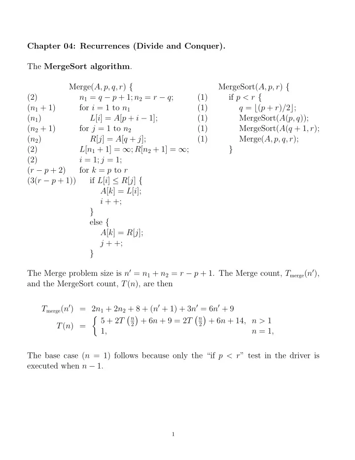
Chapter 04: Recurrences (Divide and Conquer). The MergeSort algorithm. Merge(A, p, q, r) { (2) n1 = q − p + 1; n2 = r − q; (n1 + 1) for i = 1 to n1 (n1) L[i] = A[p + i − 1]; (n2 + 1) for j = 1 to n2 (n2) R[j] = A[q + j]; (2) L[n1 + 1] = ∞; R[n2 + 1] = ∞; (2) i = 1; j = 1; (r − p + 2) for k = p to r (3(r − p + 1)) if L[i] ≤ R[j] { A[k] = L[i]; i + +; } else { A[k] = R[j]; j + +; } MergeSort(A, p, r) { (1) if p < r { (1) q = ⌊(p + r)/2⌋; (1) MergeSort(A(p, q)); (1) MergeSort(A(q + 1, r); (1) Merge(A, p, q, r); } The Merge problem size is n′ = n1 + n2 = r − p + 1. The Merge count, Tmerge(n′), and the MergeSort count, T(n), are then Tmerge(n′) = 2n1 + 2n2 + 8 + (n′ + 1) + 3n′ = 6n′ + 9 T(n) = 5 + 2T n

2

• + 6n + 9 = 2T

n

2

• + 6n + 14, n > 1

1, n = 1, The base case (n = 1) follows because only the “if p < r” test in the driver is executed when n − 1.

1

Tmerge(n′) = 2n1 + 2n2 + 8 + (n′ + 1) + 3n′ = 6n′ + 9 T(n) = 5 + 2T n

2

• + 6n + 9 = 2T

n

2

• + 6n + 14, n > 1

1, n = 1, Note: As stated, the expression for T(n) is approximate because the size of the two recursive calls to MergeSort may differ by one. If n is even, then the expression is exact; both calls have arguments of size n/2. If n is odd, the first call has an argument which is one larger than the second call.

2

The expression for T(n) is called a recurrence. T(n) = 2T n 2

• + 6n + 14.

As a first attempt to solve for T(n), we “unwind” the recurrence, restricting our attention to the subsequence n = 2k, for k = 0, 1, 2, . . .. Why the restriction? Because the progression n → n/2 → n/22 → . . . → 1 never encounters any fractions. Hence the recurrence is no longer approximate, provided n → ∞ along this particular sequence. Note the pattern: For any 2m > 1, we have T(2m) = 2T(2m−1) + 6 · 2m + 14. Starting with some n = 2k, we apply the pattern sequentially as follows. T(2k) = 2T(2k−1) + 6 · 2k + 14 = 2[2T(2k−2) + 6 · 2k−1 + 14] + 6 · 2k + 14 = 22T(2k−2) + 6 · 2 · 2k + 14(1 + 2) = 22[2T(2k−3) + 6 · 2k−2 + 14] + 6 · 2 · 2k + 14(1 + 2) = 23T(2k−3) + 6 · 3 · 2k + 14(1 + 2 + 4) = . . . = 2kT(20) + 6 · k · 2k + 14(1 + 2 + 4 + . . . + 2k−1) = 2kT(1) + 6 · k · 2k + 14

k−1

• j=0

2j = 2kT(1) + 6 · k · 2k + 14 · 2k − 1 2 − 1 = [T(1) + 14]2k + 6k2k − 14. T(1) is a constant, K1, and k = lg n. So, in terms of n, T(n) = (K1 + 14)n + 6n lg n − 14 T(n) n lg n = 6 + K1 + 14 lg n − 14 n lg n → 6 5 ≤ T(n) n lg n ≤ 7, for n = 2k sufficiently large.

3

So, T(n) ∈ Θ(n lg n), provided n grows through the restricted sequence 1, 2, 4, 8, . . .. Can we extend the result to the conventional sequence n = 1, 2, 3, . . .? If we maintain separate terms for the recursive calls, we have T(n) = T n 2

• + T
• n −

n 2

• + 6n + 14

= T n 2

• + T

n 2

• + 6n + 14.

Continuing with T(1) = K1, we compute T(n) for some initial values. T(1) = K1 T(2) = T(1) + T(1) + 6(2) + 14 = 2K1 + 26 T(3) = T(2) + T(1) + 6(3) + 14 = K1 + 2K1 + 26 + 32 = 3K1 + 58 T(4) = T(2) + T(2) + 6(4) + 14 = 4K1 + 52 + 38 = 4K1 + 90. We observe that T(n) is monotonically increasing, and we could rigorously establish this result by induction.

4

Now consider an arbitrary n, situated in an interval [2k, 2k+1) for which the above partial result holds. That is, 5 ≤ T(2k) 2k lg 2k = T(2k) 2k · k ≤ 7 5 ≤ T(2k+1) 2k+1 lg 2k+1 = T(2k+1) 2k+1 · (k + 1) ≤ 7. Starting with the monotone property of T, we reason that T(n) ≤ T(2k+1), for n ∈ [2k, 2k+1), and continue as follows. T(n) ≤ T(2k+1) ≤ 7 · [2k+1 · (k + 1)] ≤ 7 · [2k+1(2k)] = 7 · 4 · k2k = 28

• x lg x
• x=2k ≤ 28
• x lg x
• x=n = 28n lg n,

ince x lg x is also monotone increasing. So, T(n) ∈ O(n lg n) without restriction. For a lower bound, T(n) ≥ T(2k) ≥ 5 · [2k · k] ≥ 5 2 · 2k+1 · k ≥ 5 2 · 2k+1 · k + 1 2 = 5 4 · (k + 1)2k+1 = 5 4

• x lg x
• x=2k+1 ≥ 5

4

• x lg x
• x=n = 5

4n lg n. Thus, we have 5 4 ≤ T(n) n lg n ≤ 28, for all sufficiently large n. So, T(n) ∈ Ω(n lg n). Together with the upper bound above, T(n) ∈ Θ(n lg n) without restriction.

5

Master Template for recurrences Suppose T(n) > 0 is a function satisfying the following recurrence, and suppose f(n) ≥ 0. T(n) = aT n b

• + f(n), if n ≥ b

T(n) ≤ K, for 1 ≤ n < b, where a ≥ 1, b > 1, and n/b can be either ⌊n/b⌋ or ⌈n/b⌉. Then each of the following three cases provides an immediate solution for the recurrence. (a) weak glue: If ∃ǫ > 0 with f(n) = O(n[logb a]−ǫ), then T(n) = Θ(nlogb a). (b) medium glue: If f(n) = Θ(nlogb a), then T(n) = Θ(nlogb a · lg n). (c) strong glue: If ∃ǫ > 0 with f(n) = Ω(n[logb a]+ǫ) and ∃c with 0 < c < 1, af(n/b) ≤ cf(n) for all sufficiently large n, then T(n) = Θ(f(n)). Observations.

• 1. We will call f(n) the “glue function” as it represents the work required to

prepare for the recursive calls and to assemble their returned results into a solution to the overall problem.

• 2. We will call the polynomial g(n) = nlogb a the “reference function.” It represents

the work done in establishing the tree of recursive calls. In the context of algorithm analysis, the recurrence represents a recursive algorithm that divides its input into b parts and recursively considers a of them.

• 3. The variations g−(n) = n(logb a)−ǫ and g+(n) = n(logb a)+ǫ are used in cases (a) and

(c), respectively, of the template. We refer to these variations as “exponentially reduced” and “exponentially enhanced” versions of the reference.

6

Example. For MergeSort: T(n) = 2T(n/2) + f(n), where f ∈ Θ(n). This glue function then satisfies K1n ≤ f(n) ≤ K2n for all sufficiently large n. The reference function is g(n) = nlog2 2 = n1 = n. Case (a) of the master template reads: weak glue: If ∃ǫ > 0 with f(n) = O(n[logb a]−ǫ), then T(n) = Θ(nlogb a). To check out case (a), let g−(n) = n1−ǫ be an exponentially reduced version of the reference. For large n, we have f(n) g−(n) ≥ K1n n1−ǫ = K1nǫ → ∞, which implies f(n) = O(n1−ǫ) for any ǫ > 0. Case (a) fails. Case (b) of the master template reads: medium glue: If f(n) = Θ(nlogb a), then T(n) = Θ(nlogb a · lg n). To check out case (b), we investigate the ratio of the glue function to the reference function: 0 < K1 ≤ K1n n ≤ f(n) g(n) ≤ K2n n = K2 < ∞, which implies f ∈ Θ(g). Case (b) succeeds, and therefore T(n) = Θ(n lg n).

7

Case (c) of the master template reads: strong glue: If ∃ǫ > 0 with f(n) = Ω(n[logb a]+ǫ) and ∃c with 0 < c < 1, af(n/b) ≤ cf(n) for all sufficiently large n, then T(n) = Θ(f(n)). In the problem at hand, if g+ = n1+ǫ any exponentially enhanced reference, we have f(n) g+(n) ≤ K2n n1+ǫ = K2 nǫ → 0. For any ǫ > 0, there is no possible positive lower bound under f/g+. Therefore f ∈ Ω(g+) and case (c) fails. In general, you can check out the cases in the master template in any order. If you find one that works, then you can ignore all of the others. The homework asks you to prove that the three cases of the master template are mutually exclusive. That is, if one of the cases succeeds, the other two must fail.

8

• Example. Suppose

T(n) = 2T(n/3) + √n. We have f(n) = n1/2, and g(n) = nlog3 2. Note that 0.5 = log3 31/2 = log3 1.732 < log3 2. Choose ǫ as shown above. Then f(n) g−(n) = n1/2 n(log3 2)−ǫ → 0. Thus f ∈ o(g−), which implies f ∈ O(g−), which enables case (a), which gives T(n) = Θ(nlog3 2).

9

• Example. T(n) = 49T(n/25) + n3/2 lg n. Here a = 49, b = 25, so log25 49 = 1.209.

The reference is g(n) = n1.209. The glue is f(n) = n1.5 lg n. f(n) g+(n) = n1.5 log2 n n1.209+ǫ = n0.291−ǫ log2 n → ∞ as n → ∞ for any 0 < ǫ < 0.291. That is, f(n) = ω(n1.209+ǫ), which implies f(n) = Ω(n1.209+ǫ). This leads to a possible application of case (c) of the template. There is, however, a regularity condition that must be satisfied: af(n/b) ≤ cf(n) for some constant 0 < c < 1 and all sufficiently large n. In the problem at hand, af(n/b) = 49f(n/25) = 49 · n 25 3/2 · lg n 25 = 49n3/2 (25)3/2 · [(lg n) − (lg 25)] ≤ 49 125n3/2 lg n = 49 125f(n). Consequently, the value c = 49/125 satisfies the regularity condition. Then T(n) = Θ(f(n)) = Θ(n3/2 lg n) via case (c) of the template.

10

Maximum subarray problem: given a vector of real numbers, find a contiguous segment with the largest sum. Output the lower and upper indices of the chosen segment and the resulting optimal sum. Observations:

• 1. If the array contains only nonnegative numbers, choose the entire array.
• 2. If the array contains only negative numbers, choose the negative number closest

to zero in an array of length 1.

• 3. If the array contains both positive and negative numbers, divide it in half.

The optimal segment is in the lower array, in the upper array, or it crosses the boundary between the two. (low, high, sum) = MaxSubArray(A, 1, length(A)); MaxSubArray(A, low, high) { if (low = high) return (low, low, A[low]); mid = (low + high)/2; (leftLow, leftHigh, leftSum) = MaxSubArray(A, low, mid); (rightLow, rightHigh, rightSum) = MaxSubArray(A, mid + 1, high); (crossLow, crossRight, crossSum) = CrossSubArray(A, low, mid, high); if (leftSum ≥ rightSum) and (leftSum ≥ crossSum) return (leftLow, leftHigh, leftSum); if (rightSum ≥ leftSum) and (rightSum ≥ crossSum) return (rightLow, rightHigh, rightSum); else return (crossLow, crossHigh, crossSum); } minimum count = 2. maximum count = 8 + work in CrossSubArray + work in two recursive calls.

11

CrossSubArray(A, low, mid, high) { leftSum = −∞; sum = 0; for k = mid downto low { sum = sum + A[k]; if (sum > leftSum) { leftSum = sum; maxLeft = k; } } rightSum = −∞; sum = 0; for k = mid + 1 to high { sum = sum + A[k]; if (sum > rightSum) { rightSum = sum; maxRight = k; } } return (maxLeft, maxRight, leftSum + rightSum); } count = 7+(3 to 5)·n′, where n′ = high − low +1 is the length of the subproblem under analysis. T(n′) = 8 + 7 + (3 to 5)n′ + 2T(n′/2) = 2T(n′/2) + (3 to 5)n + 15 = 2T(n′/2) + f(n) T(n) = 2T(n/2) + f(n), n > 1 2, n = 1

12

Check the master template: Suppose T(n) > 0 is a nondecreasing function satisfying the following recurrence, and suppose f(n) ≥ 0. Also, T(n) = aT n b

• + f(n), if n ≥ b

T(n) ≤ K, for 1 ≤ n < b, where a ≥ 1, b > 1, and n/b can be either ⌊n/b⌋ or ⌈n/b⌉. Then each of the following three cases provides an immediate solution for the recurrence. (a) If ∃ǫ > 0 with f(n) = O(n[logb a]−ǫ), then T(n) = Θ(nlogb a). (b) If f(n) = Θ(nlogb a), then T(n) = Θ(nlogb a · lg n). (c) If ∃ǫ > 0 with f(n) = Ω(n[logb a]+ǫ) and ∃c with 0 < c < 1, af(n/b) ≤ cf(n) for all sufficiently large n, then T(n) = Θ(f(n)). For MaximumSubarray: T(n) = 2T(n/2) + f(n), with f(n) ∈ Θ(n); reference function is g(n) = nlog2 2 = n. So, f ∈ Θ(g), which enables case (b) of the Master Template. T(n) = Θ(n lg n).

13

Matrix multiplication: Given two n × n matrices, [aij] and [bij], their product is [cij], where cij =

n

• k=1

aikbkj. MatrixMultiply(a, b) { for i = 1 to n n + 1 for j = 1 to n n(n + 1) for k = 1 to n n2(n + 1) c[i][j] = a[i][k] ∗ b[k][j]; n3 } Have T(n) = (n + 1) + n(n + 1) + n2(n + 1) + n3 = 2n3 + 2n2 + 2n + 1 = Θ(n3). Recursive approach: for n = 2k, divide factors into four pieces. C11 C12 C21 C22

• =

A11 A12 A21 A22

• ·

B11 B12 B21 B22

• C11 = A11B11 + A12B21

C12 = A11B12 + A12B22 C21 = A21B11 + A22B21 C22 = A21B12 + A22B22 But, can isolate components by passing row and column boundaries to recursive calls, and merge results of recursive calls by doing 4(n/2)(n/2) = n2 additions. Then, T(n) = 8T(n/2) + n2. Glue is n2; reference is nlog2 8 = n3. Then n2/n3 = 1/n → 0, implying n2 = o(n3), which in turn implies n2 = O(n3), which enables case (a). Therefore T(n) = Θ(n3).

14

• 1. Notice that addition is much less expensive than multiplication. Given two

n × n matrices, [aij] and [bij], their sum is [cij], where cij = aij + bij. MatrixAdd(a, b) { for i = 1 to n n + 1 for j = 1 to n n(n + 1) c[i][j] = a[i][j] + b[i][j]; n2 } T(n) = (n + 1) + n(n + 1) + n2 = 2n2 + 2n + 1 = Θ(n2).

• 2. Very clever observation for case of 2×2 matrices: 8 multiplications, 4 additions.

A = a b c d

• B =

e f g h

• AB =

ae + bg af + bh ce + dg cf + dh

• becomes 7 multiplication and (about) 18 additions/subtractions.

AB =      −(a + b)h + d(g − e) + (a + d)(e + h) a(f − h) + (a + b)h +(b − d)(g + h) (c + d)e + d(g − e) a(f − h) − (c + d)e + (a + d)(e + h) −(a − c)((e + f)      7 multiplications are: (a + b)h d(g − e) (a + d)(e + h) (b − d)(g + h) a(f − h) (c + d)e (a − c)(e + f)

15

Strassen’s Method, for n = 2k. Step 1: Divide the input matrix into four (n/2) × (n/2) matrices as above. Θ(1), that is, constant time via index calculations. Step 2: Compute 10 matrices S1, . . . , S10, each (n/2) × (n/2), in Θ(n2) time. These correspond to the factors in the 7 multiplications above: (a + b), (g − e), (a + d), (e + h), (b − d), (g + h), (f − h), (c + d), (a − c), (e + f) Step 3: Recursively compute 7 matrix products: P1, . . . , P7, each of size (n/2) × (n/2). These correspond to the 7 multiplications themselves: (a + b)h, d(g − e), (a + d)(e + h), (b − d)(g + h), a(f − h), (c + d)e, (a − c)(e + f) Step 4: Create the components C11, C12, C21, C22 by adding and subtracting various combinations of the matrix products in Θ(n2) time. T(n) = 7T(n/2) + Θ(n2) Reference function is nlog2 7 = n2.8074. Glue function is f(n) = Θ(n2). f(n) n2.8074−ǫ ≤ K2n2 n2.8074−ǫ = K2 n0.8074−ǫ → 0, for 0 < ǫ < 0.8074. f(n) = o(n2.8074−ǫ), which implies f(n) = O(n2.8074−ǫ), which enables case(a). T(n) = Θ(n2.8074). Observation: For matrices which are not of size equal to a power of 2, pad with zeros to the next power of two. Desired product appears in the upper left corner

• f the larger product.

16

Alternatives to the master template. (a) Induction (also called back-substitution) Step 1: Guess the form of the solution, normally by examining small cases. Step 2: Prove the form correct via induction. Example: T(n) = 2T n

2

• + n, n ≥ 2

1, n = 1 To facilitate our guess, consider just n = 2k, rather than a general integer n. In this case, the round-down operation has no effect. T(1) = 1 T(2) = 2T(1) + 2 = 4 = 21(1 + 1) T(4) = 2T(2) + 4 = 12 = 22(2 + 1) T(8) = 2T(4) + 8 = 32 = 23(3 + 1) T(16) = 2T(8) + 16 = 80 = 24(4 + 1) It appears T(2k) = 2k(k +1). In terms of n = 2k, we have T(n) = n(1+lg n) = n lg(2n) when n is a power of 2. We now guess that T(n) ≤ cn lg(2n), for n ≥ 2 (to avoid a right-hand-side zero) and an appropriately chosen c > 1. We start an induction proof by working out the first few cases, say n = 2, 3, 4, and choosing a c > 1 that works for all of those cases. Then, for larger n, we argue T(n) = 2T(⌊n/2⌋) + n ≤ 2c⌊n/2⌋ lg(2⌊n/2⌋) + n ≤ 2c n 2

• lg
• 2 · n

2

• + n

= cn[(lg 2n) − 1] + n = cn lg(2n) + n(1 − c) ≤ cn lg(2n), the last since 1 − c < 0. Also, since n lg(2n) = n(1+lg n) ≤ 2n lg n, for n ≥ 2, we have T(n) ≤ 2cn lg n. We conclude T(n) = O(n lg n).

17

(b) Recursion-trees Consider the recurrence: T(n) = 3T(⌊n/4⌋) + n2. Our goal is to obtain a general form for the solution that we can verify via induction as in part (a)

• above. Working with the sequence n = 4k for k = 0, 1, . . . is convenient because

the round-down operation does not introduce any fractions. However, instead

• f developing the recurrence algebraically, we draw a tree that illustrates the

various subproblems considered. Each node make three recursive calls to its children. The recursive calls them- selves constitute a constant amount of work — establishing the stack frame and copying argument pointers — that does not grow with the size of the problem. However, each node expends m2 work, where m is the size of the node’s input, in processing the recursive returns into a package to return to its caller. This latter processing does grow with the size of the problem. In the tree above, the right edge totals the processing associated with the nodes

• n a given level. To obtain a grand total over all nodes, we sum the sub-totals

associated with each level: T(n) =

log4 n

• j=0

3j n 4j 2 = n2

log4 n

• j=0

3 16 j ≤ n2

∞

• j=0

3 16 j = n2 1 − 3/16 = 16 13 · n2 = Θ(n2). We can then conjecture T(n) ≤ cn2 for some appropriate constant c and con- tinue with a proof by induction.

18

The master template for recurrences.

• 1. Statement of the theorem.

Suppose T(n) > 0 is a nondecreasing function satisfying the following recur- rence, and suppose f(n) ≥ 0. Also, T(n) = aT n b

• + f(n), if n ≥ b

T(n) ≤ K, for 1 ≤ n < b, where a ≥ 1, b > 1, and n/b can be either ⌊n/b⌋ or ⌈n/b⌉. Then each of the following three cases provides an immediate solution for the recurrence. (a) If ∃ǫ > 0 with f(n) = O(n[logb a]−ǫ), then T(n) = Θ(nlogb a). (b) If f(n) = Θ(nlogb a), then T(n) = Θ(nlogb a · lg n). (c) If ∃ǫ > 0 with f(n) = Ω(n[logb a]+ǫ) and ∃c with 0 < c < 1, af(n/b) ≤ cf(n) for all sufficiently large n, then T(n) = Θ(f(n)).

19

• 2. Proof of Case (a): If ∃ǫ > 0 with f(n) = O(n[logb a]−ǫ), then T(n) = Θ(nlogb a).

We are interested in the asymptotic growth of T(n) as n → ∞. To this end, we first consider a special case where n approaches ∞ through a constrained sequence: n = bk, for k = 0, 1, 2, . . .. Along this sequence k = logb n and the general recurrence pattern is, for any exponent t > 0, T(bt) = aT(bt−1) + f(bt), while the base case corresponds to t = 0: T(b0) = T(1), some constant. We expand the recurrence, starting with the generic n = bk. T(bk) = aT(bk−1) + f(bk) = a

• aT(bk−2) + f(bk−1)
• + f(bk) = a2T(bk−2) + af(bk−1) + f(bk)

= a2 aT(bk−3) + f(bk−2)

• + af(bk−1) + f(bk)

= a3T(bk−3) + a2f(bk−2) + af(bk−1) + f(bk) . . . = akT(b0) + ak−1f(b1) + ak−2f(b2) + . . . + a0f(bk) That is, T(bk) = akT(1) +

k−1

• j=0

ajf(bk−j) = akT(1) +

k

• j=1

ak−jf(bj). (1)

20

Since f is a positive function, we immediately have T(n) ≥ T(1) · ak = T(1) · alogb n. Considering the following useful rearrangement, n = blogb n nlogb a =

• blogb nlogb a = b(logb n)(logb a) =
• blogb alogb n = alogb n,

(2) we now have T(n) ≥ T(1) · nlogb a and therefore T(n) = Ω(nlogb a) along the constrained sequence n = bk. Note that we have not used the hypothesis: ∃ǫ > 0 with f(n) = O(n[logb a]−ǫ). ?? Is this partial result true for all three cases?

• Yes. In case (b), the result is T(n) = Ω(nlogb a · lg n), a tighter lower bound.

In case (c), the result is T(n) = Ω(f) ≥ Ω(n(logb a)+ǫ), a yet tighter lower bound.

21

Returning to Equation (1), we now pursue an upper bound. Since T(1) is just another constant, say K1, we start with T(bk) = K1ak +

k

• j=1

ak−jf(bj). Since we know that f(n) = O(n[logb a]−ǫ), we can bound the f(bj) terms when j is large. Specifically, ∃k1, K2 with n ≥ bk1 implying f(n) ≤ K2n[logb a]−ǫ. To use this constraint, we break the sum above into two components: T(bk) = K1ak +

k1

• j=1

ak−jf(bj) +

k

• j=k1+1

ak−jf(bj), for k ≥ k1.

22

Now let K3 = max1≤j≤k1 f(bj), a constant that allows us to combine the first sum with the K1ak term. Specifically, since a ≥ 1, we have T(bk) ≤ K1ak + K3

k1

• j=1

ak−j +

k

• j=k1+1

ak−jf(bj) ≤ K1ak + K3ak

k1

• j=1

a−j +

k

• j=k1+1

ak−jf(bj) ≤ K1ak + K3ak

k1

• j=1

(1) +

k

• j=k1+1

ak−jf(bj) = (K1 + k1K3)ak +

k

• j=k1+1

ak−jf(bj). In the remaining sum, j > k1, which implies bj > bk1 and therefore f(bj) ≤ K2

• bj[logb a]−ǫ = K2b−jǫ · bj logb a = K2

1 bǫ j ·

• blogb aj = K2

1 bǫ j · aj T(bk) ≤ (K1 + k1K3)ak +

k

• j=k1+1

ak−jK2aj 1 bǫ j = (K1 + k1K3)ak + K2ak

k

• j=k1+1

1 bǫ j ≤ (K1 + k1K3)ak + K2ak

∞

• j=0

1 bǫ j = (K1 + k1K3)ak + K2ak 1 − (1/bǫ). The last reduction obtains because b > 1, ǫ > 0, which implies that (1/bǫ) < 1 and the infinite geometric series converges.

23

Therefore, we have T(bk) ≤

• K1 + k1K3 +

K2 1 − (1/bǫ)

• ak =
• K1 + k1K3 +

K2 1 − (1/bǫ)

• alogb n

=

• K1 + k1K3 +

K2 1 − (1/bǫ)

• nlogb a,

where the last reduction uses Equation (2). We now have T(n) = O(nlogb a) along the constrained sequence n = bk. Combining this upper bound with the lower bound from above, we have T(n) = Θ(nlogb a) along the constrained sequence n = bk. Moreover, on this constrained sequence, any floor or ceiling functions in the recurrence have no effect. That is, the analysis to this point is valid whether the recurrence is either of the forms T(n) = aT n b

• + f(n)

T(n) = aT n b

• + f(n),

(3)

• r any combination of floor and ceiling operations on the a recursive arguments.

24

We now exploit the fact that T(n) is nondecreasing to show that T(n) = O(nlogb a) without the restriction to the constrained sequence n = bk. Again, the particular form of the recurrence (Equations (3)) will not enter into the analysis. Introducing new constants, the constrained result is ∃k2, K4, K5 such that k ≥ k2 implies K4(bk)logb a ≤ T(bk) ≤ K5(bk)logb a K4

• blogb ak ≤ T(bk) ≤ K5
• blogb ak

K4ak ≤ T(bk) ≤ K5ak Now, for an unconstrained n ≥ bk2, we have, for some j ≥ k2, bj ≤ n < bj+1. The nondecreasing nature of T forces T(n) ≤ T(bj+1) ≤ K5aj+1 = K5a · aj = K5a ·

• blogb aj = K5a ·
• bjlogb a

= K5a

• xlogb a
• x=bj ≤ K5a
• xlogb a
• x=n = K5a · nlogb a.

That is, T(n) = O(nlogb a) without restriction. Similarly, T(n) ≥ T(bj) ≥ K4aj = K4 a · aj+1 = K4 a ·

• blogb aj+1 = K4

a ·

• bj+1logb a

= K4 a

• xlogb a
• x=bj+1 ≥ K4

a

• xlogb a
• x=n = K4

a · nlogb a, which implies T(n) = Ω(nlogb a) without restriction. Combining the two results, we have the desired relationship: T(n) = Θ(nlogb a).

25