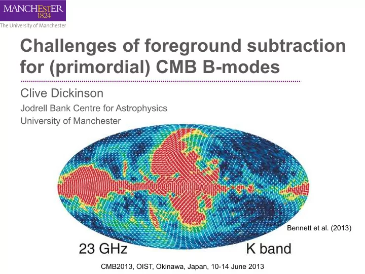
Challenges of foreground subtraction for (primordial) CMB B-modes - PowerPoint PPT Presentation

Challenges of foreground subtraction for (primordial) CMB B-modes Clive Dickinson Jodrell Bank Centre for Astrophysics University of Manchester Bennett et al. (2013) CMB2013, OIST, Okinawa, Japan, 10-14 June 2013

Component separation for B-modes • Separate primordial CMB emission from (l~5 and l~90) • Diffuse Galactic foregrounds • Other foregrounds probably dealt with in other ways (e.g. source detection/ masking, power spectrum templates, source detection, statistical estimators etc.) • Extragalactic sources (Poisson) • CIB (clustering) • SZ clusters • CMB lensing • Propagate uncertainties to map/power spectra/cosmological parameters • If possible: • Fit for residual monopoles/dipoles • Deal with bandpasses (“colour corrections”) • Deal with other systematics (e.g. calibration - see e.g. Dick et al. 2011) • Separate foregrounds into (multiple) individual components (astrophysics)

Extragalactic sources • Extragalactic sources are not very polarized 1Jy • ~ 3.5% for radio sources (Battye et al. 2011) 0.1Jy • <~1% in FIR for star-forming galaxies 0.01Jy r=0.1 • 1.5% Upper limit of for Arp220 (Seiffert et al. 2006) r=0.01 r=0.001 • Power is relatively small at freqs > 30 GHz • Subtract/mask the brightest sources • Statistically correct the residual sources • N.B. CIB will be < 1% polarized but still important • Correlated on large angular scales (~1 deg) • Polarization does *not* average out (variance does not average) Battye, ..., Dickinson et al. (2011)

Large scale polarized foregrounds • Diffuse polarized foregrounds dominate at l<100 Component Spectrum Polariza1on ¡ References frac1on Synchrotron Power-­‑law, ¡β~-­‑3.1, ¡possible ¡ ~15-­‑20% ¡ Page ¡et ¡al. ¡(2007), ¡Kogut ¡et ¡al. ¡(2007), ¡ Macellari ¡et ¡al. ¡(2011) curvature (up ¡to ¡~50%) Thermal ¡dust Modified ¡black-­‑body, ¡possibly ¡ ~5% ¡ Ponthieu ¡et ¡al. ¡(2005), ¡Planck ¡ CollaboraUon, ¡ESLAB ¡conference ¡(2013). 2 ¡components/flaJening ¡at ¡ (up ¡to ¡~15+%!) frequencies ¡<300 ¡GHz Planck ¡papers ¡to ¡come ¡out ¡soon! MagneUc ¡ Similar ¡to ¡thermal ¡dust, ¡but ¡ Variable Draine ¡& ¡Lazarian ¡(1999), ¡Draine ¡& ¡ Hensley ¡(2013) flaJer ¡index ¡at ¡frequencies ¡ dipole? (up ¡to ¡~35%!?) ~100 ¡GHz Peaked ¡spectrum ¡~10-­‑60 ¡GHz. Lazarian ¡& ¡Draine ¡(2000), ¡Dickinson ¡ AME ¡ <~1% (2011), ¡Lopez-­‑Caraballo ¡et ¡al. ¡(2011), ¡ Macellari ¡et ¡al. ¡(2011), ¡Rubino-­‑MarUn ¡et ¡ (spinning ¡dust) al. ¡(2012) Free-­‑free Power-­‑law ¡β~-­‑2.14 ¡with ¡ <~1% Rybicki ¡& ¡Lightman ¡(1979), ¡KeaUng ¡et ¡al. ¡ (1998), ¡Macellari ¡et ¡al. ¡(2011) posiUve ¡curvature ¡(steepening ¡ at ¡frequencies ¡>~100 ¡GHz)

Temperature vs Polarization • Foregrounds not a major issue for intensity • 40 - 250 GHz relatively clean at high latitudes • Still “see” CMB at 20 GHz and 353 GHz !!! • Similar levels for E-modes • CMB and foregrounds polarized at ~10% level • Low-l (l<10) significantly contaminated • CMB B-modes (l<100) much more contaminated by foregrounds • CMB < 1% polarized • Foregrounds ~10% polarized! Planck Collaboration I (2013)

Intensity foregrounds Details of intensity foregrounds are quite complex! But quite interesting astrophysically speaking! Polarization may well be simpler!?! Bennett et al. (2013)

Intensity foregrounds vs CMB Only very largest scales, including Galactic plane, which are strongly affected by diffuse foregrounds (TT) Dunkley et al. (2009) U.S. Decadal review white paper (based on Planck Sky Model simulations; see Delabrouille et al. (2013)

Polarized foregrounds vs CMB B-modes For r=0.01, foregrounds dominate CMB almost everywhere at all frequencies on scales >1 deg r=0.01 Dunkley et al. (2009) U.S. Decadal review white paper (based on Planck Sky Model simulations; see Delabrouille et al. (2013)

Component separation methods • Many methods/algorithms/codes out there! (see next slide) • 3 broad categories • 1. Parametric / non-blind (e.g. pixel fitting, external template fitting) • 2. Semi-blind (use some external info but not reliant e.g. SMICA, CCA) • 3. Blind (e.g. ILC, ICA, PCA, Neural networks) • Most successful / popular so far have been simple ones! • Template fitting, ILC, parametric fitting... • Do not want to change noise properties of maps • Important to fully propagate errors (using likelihood) • Simple, linear methods are preferred! (see Komatsu talk) • But times are changing... • c.f. Planck Collaboration XII (2013):SMICA, GMCA, NILC, Commander-Ruler

(some) Component separation methods DISCLAIMER: this list is not comprehensive and some algorithms grouped together (but are quite different) Type Codes ¡/ ¡implementa1ons Method ¡/ ¡assump1ons References ILC Pixel ¡based ¡ILC, ¡NILC, ¡ Internal ¡Linear ¡CombinaUon ¡-­‑ ¡CMB ¡spectrum ¡ BenneJ ¡et ¡al. ¡(2003), ¡Delabrouille ¡et ¡ Constrained ¡ILC, ¡MILCA conserved al. ¡(2007), ¡Remazeilles ¡et ¡al. ¡(2011) ¡, ¡ Hurier ¡et ¡al. ¡(2010) ICA FastICA, ¡AltICA, ¡JADE Independent ¡Component ¡Analysis ¡-­‑ ¡Gaussian ¡ Hyvarinen ¡(1999), ¡Cardoso ¡(1999), ¡ CMB/non-­‑Gaussian ¡foregrounds Maino ¡et ¡al. ¡(2002) Sparsity GMCA, ¡PCA, ¡Neural ¡networks Foregrounds ¡described ¡by ¡few ¡numbers ¡in ¡ Bobin ¡et ¡al. ¡(2007, ¡2013), ¡Leach ¡et ¡al. ¡ certain ¡basis ¡set ¡(e.g. ¡PCA) (2005), ¡Norgard-­‑Nielsen ¡(2008) Template ¡fikng Linear ¡sum ¡of ¡spaUal ¡ Linear ¡sum ¡of ¡spaUal ¡templates ¡ Bennet ¡et ¡al. ¡(2003), ¡Page ¡et ¡al. ¡ templates, ¡WIFIT, ¡SEVEM (2007), ¡Hansen ¡et ¡al. ¡(2006), ¡ (external ¡or ¡internal ¡templates) MarUnez-­‑Gonzalez ¡et ¡al. ¡(2003) Spectral ¡matching SMICA EsUmates ¡model ¡parameters ¡(mixing ¡ Delabrouille ¡et ¡al. ¡(2003), ¡Cardoso ¡et ¡ al. ¡(2008) coefficients/power ¡spectrum) ¡using ¡2nd ¡order ¡ staUsUcs ¡(correlaUons). ¡Then ¡Wiener ¡filtering. ¡ Correlated ¡ CCA CorrelaUons ¡used ¡to ¡esUmate ¡mixing ¡matrix, ¡ Bedini ¡et ¡al. ¡(2003), ¡Bonaldi ¡et ¡al. ¡ Components then ¡Wiener ¡filtering ¡soluUon (2006) Pixel-­‑based ¡frequency ¡ Commander, ¡MEM, ¡Miramare, ¡ Pixel-­‑based ¡parametric ¡fikng. ¡Simple ¡models ¡in ¡ Eriksen ¡et ¡al. ¡(2006, ¡2008), ¡Leach ¡et ¡ spectral ¡fikng Galclean ¡(MCMC) frequency ¡space. ¡MCMC/Gibbs ¡sampling. al. ¡(2008), ¡Stompor ¡et ¡al. ¡(2009), ¡ Dunkley ¡et ¡al. ¡(2009) Power ¡spectrum ¡ FastMEM, ¡Planck ¡likelihood Mask ¡and ¡then ¡fit ¡power-­‑law ¡in ¡the ¡power ¡ Hobson ¡et ¡al. ¡(1998), ¡Stolyrov ¡et ¡al. ¡ fikng spectrum (2002), ¡Planck ¡CollaboraUon ¡(2013) Hierarchical ¡Bayesian ¡ Hierarchical ¡Bayesian ¡fikng a Morishima ¡poster fikng Blind (green), semi-blind (yellow) and non-blind (orange)

Forecasts for B-modes • Planck should be able to detect r ~ 0.05-0.1 (Efstathiou & Gratton 2009, Betoule et al. 2009, Bonaldi & Ricciardi 2011, Armitage-Caplan et al. 2011) • Foregrounds become significant limitation for r<0.1 • Typically 30-100% increase in errors due to component separation • BUT, several studies have shown r~0.001 can be reached (Dunkley et al. 2009, Betoule et al. 2009, Katayama & Komatsu 2011) Dunkley et al. (2009) U.S. Decadal review white paper

Potential issues • Are polarized foregrounds so simple? • Thermal dust polarization possibly more polarized than first thought • Subtle spectral variations in synchrotron/dust • AME polarization ? • Magnetic dust polarization • Calibration • Gain calibration (e.g. Dick et al. 2011) • Offsets (e.g. Eriksen et al. 2008) • Bandpass mis-match • Effective frequencies (colour corrections) • Other systematics • Line contamination! (c.f. CO for Planck!) • Polarization leakage (I->Q,U) • Polarization angle calibration • 1/f (striations) • Spillover (sidelobes) • .....

Foreground modelling examples • For Planck (Armitage-Caplan et al. 2011): • ~1% polarized free-free or spinning dust has negligible effect on Planck • Curvature of synchrotron can bias r by ~1 σ (r~0.03) • Mis-matches in synchrotron spectral index can bias r by up to ~3 σ • For CMBpol/EPIC/CORE/LiteBird etc. we will be much more sensitive to foreground modelling errors! • see also Betoule et al. (2009) Armitage-Caplan, Dunkley, CD, Eriksen (2012)