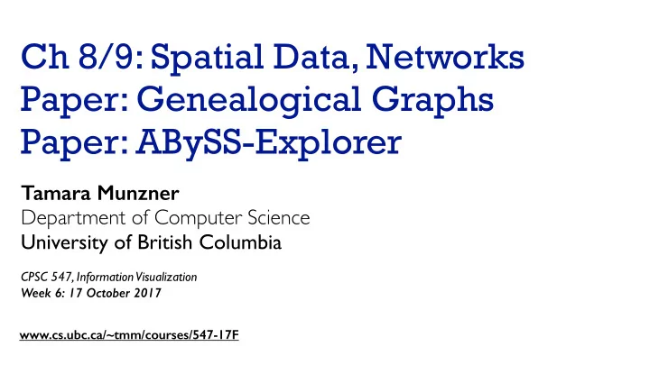
ch 8 9 spatial data networks paper genealogical graphs
play

Ch 8/9: Spatial Data, Networks Paper: Genealogical Graphs Paper: - PowerPoint PPT Presentation

Ch 8/9: Spatial Data, Networks Paper: Genealogical Graphs Paper: ABySS-Explorer Tamara Munzner Department of Computer Science University of British Columbia CPSC 547, Information Visualization Week 6: 17 October 2017


  1. Ch 8/9: Spatial Data, Networks Paper: Genealogical Graphs Paper: ABySS-Explorer Tamara Munzner Department of Computer Science University of British Columbia CPSC 547, Information Visualization Week 6: 17 October 2017 www.cs.ubc.ca/~tmm/courses/547-17F

  2. News • marks for previous 2 weeks published –first week was pass/fail for having anything –now more fine-grained guidance about expectations with comments • if you didn’t get full credit –in general: don’t just summarize • today –pitches first –Q&A, lecture second 2

  3. Ch 8: Arrange Spatial Data 3

  4. Arrange spatial data Use Given Geometry Geographic Other Derived Spatial Fields Scalar Fields (one value per cell) Isocontours Direct Volume Rendering Vector and Tensor Fields (many values per cell) Flow Glyphs (local) Geometric (sparse seeds) Textures (dense seeds) Features (globally derived) 4

  5. Idiom: choropleth map • use given spatial data –when central task is understanding spatial relationships • data –geographic geometry –table with 1 quant attribute per region • encoding http://bl.ocks.org/mbostock/4060606 –use given geometry for area mark boundaries –sequential segmented colormap [more later] –(geographic heat map) 5

  6. Population maps trickiness • beware! • absolute vs relative again • population density vs per capita • investigate with Ben Jones Tableau Public demo • http://public.tableau.com/profile/ ben.jones#!/vizhome/PopVsFin/PopVsFin 
 Are Maps of Financial Variables just Population Maps? • yes, unless you look at per capita (relative) numbers [ https://xkcd.com/1138 ] 6

  7. Idiom: Bayesian surprise maps • use models of expectations to highlight surprising values • confounds (population) and variance (sparsity) [Surprise! Bayesian Weighting for De-Biasing Thematic Maps. Correll and Heer. Proc InfoVis 2016] https://medium.com/@uwdata/surprise-maps-showing-the-unexpected-e92b67398865 https://idl.cs.washington.edu/papers/surprise-maps/ 7

  8. Idiom: topographic map • data –geographic geometry –scalar spatial field • 1 quant attribute per grid cell • derived data –isoline geometry • isocontours computed for specific levels of scalar values Land Information New Zealand Data Service 8

  9. Idioms: isosurfaces, direct volume rendering • data –scalar spatial field • 1 quant attribute per grid cell • task –shape understanding, spatial relationships [Interactive Volume Rendering Techniques. Kniss. Master’s thesis, University of Utah Computer Science, 2002.] • isosurface D –derived data: isocontours computed for F specific levels of scalar values C • direct volume rendering –transfer function maps scalar values to B color, opacity E [Multidimensional Transfer Functions for Volume Rendering. Kniss, Kindlmann, and Hansen. In The Visualization Handbook, edited by Charles Hansen and Christopher Johnson, pp. 189–210. Elsevier, 2005.] 9

  10. Vector and tensor fields • data –many attribs per cell • idiom families –flow glyphs • purely local –geometric flow • derived data from tracing particle trajectories [Comparing 2D vector field visualization methods: A user study. Laidlaw et al. IEEE Trans. • sparse set of seed points Visualization and Computer Graphics (TVCG) 11:1 (2005), 59–70.] –texture flow • derived data, dense seeds –feature flow • global computation to detect features – encoded with one of methods above [Topology tracking for the visualization of time-dependent two-dimensional flows. Tricoche, Wischgoll, Scheuermann, and Hagen. Computers & Graphics 26:2 (2002), 249–257.] 10

  11. Vector fields • empirical study tasks –finding critical points, identifying their types –identifying what type of critical point is at a specific location –predicting where a particle starting at a specified point will end up (advection) [Comparing 2D vector field visualization methods: A user study. Laidlaw et al. IEEE Trans. Visualization and Computer Graphics (TVCG) 11:1 (2005), 59–70.] [Topology tracking for the visualization of time-dependent two-dimensional flows. Tricoche, Wischgoll, Scheuermann, and Hagen. Computers & Graphics 26:2 (2002), 249–257.] 11

  12. Idiom: similarity-clustered streamlines • data –3D vector field • derived data (from field) –streamlines: trajectory particle will follow • derived data (per streamline) –curvature, torsion, tortuosity –signature: complex weighted combination –compute cluster hierarchy across all signatures –encode: color and opacity by cluster • tasks –find features, query shape [Similarity Measures for Enhancing Interactive Streamline Seeding. • scalability McLoughlin,. Jones, Laramee, Malki, Masters, and. Hansen. IEEE Trans. Visualization and Computer Graphics 19:8 (2013), 1342–1353.] –millions of samples, hundreds of streamlines 12

  13. Ch 9: Arrange Network Data 13

  14. Arrange networks and trees Node–Link Diagrams Connection Marks NETWORKS TREES Adjacency Matrix Derived Table NETWORKS TREES Enclosure Containment Marks NETWORKS TREES 14

  15. Idiom: force-directed placement • visual encoding –link connection marks, node point marks • considerations –spatial position: no meaning directly encoded • left free to minimize crossings –proximity semantics? • sometimes meaningful • sometimes arbitrary, artifact of layout algorithm • tension with length – long edges more visually salient than short • tasks –explore topology; locate paths, clusters • scalability –node/edge density E < 4N http://mbostock.github.com/d3/ex/force.html 15

  16. Idiom: sfdp (multi-level force-directed placement) • data –original: network –derived: cluster hierarchy atop it • considerations –better algorithm for same encoding technique • same: fundamental use of space • hierarchy used for algorithm speed/quality but [Efficient and high quality force-directed graph drawing. not shown explicitly Hu. The Mathematica Journal 10:37–71, 2005.] • (more on algorithm vs encoding in afternoon) • scalability –nodes, edges: 1K-10K –hairball problem eventually hits 16 http://www.research.att.com/yifanhu/GALLERY/GRAPHS/index1.html

  17. Idiom: adjacency matrix view • data: network –transform into same data/encoding as heatmap • derived data: table from network [NodeTrix: a Hybrid Visualization of Social Networks. Henry, Fekete, and McGuffin. IEEE TVCG (Proc. InfoVis) 13(6):1302-1309, 2007.] –1 quant attrib • weighted edge between nodes –2 categ attribs: node list x 2 • visual encoding –cell shows presence/absence of edge • scalability –1K nodes, 1M edges [Points of view: Networks. Gehlenborg and Wong. Nature Methods 9:115.] 17

  18. Connection vs. adjacency comparison • adjacency matrix strengths –predictability, scalability, supports reordering –some topology tasks trainable • node-link diagram strengths –topology understanding, path tracing –intuitive, no training needed http://www.michaelmcguffin.com/courses/vis/patternsInAdjacencyMatrix.png • empirical study –node-link best for small networks –matrix best for large networks • if tasks don’t involve topological structure! [On the readability of graphs using node-link and matrix-based representations: a controlled experiment and statistical analysis. Ghoniem, Fekete, and Castagliola. Information Visualization 4:2 (2005), 114–135.] 18

Download Presentation
Download Policy: The content available on the website is offered to you 'AS IS' for your personal information and use only. It cannot be commercialized, licensed, or distributed on other websites without prior consent from the author. To download a presentation, simply click this link. If you encounter any difficulties during the download process, it's possible that the publisher has removed the file from their server.

Recommend


More recommend