Cash Transfers, Household Composition, and Human Capital Accumulation - - PDF document

1 Cash Transfers, Household Composition, and Human Capital Accumulation in sub- Saharan Africa: Experimental Evidence from Lesotho, Malawi, and Zambia Jacobus de Hoop1 Sudhanshu Handa2 Ramaele Moshoeshoe3 VERSION 2: SEPTEMBER 2017 NOT TO BE SHARED OR QUOTED Abstract: This paper presents experimental evidence on the effects of large-scale, government-run, unconditional cash transfer programs in Lesotho, Malawi, and Zambia on children’s

• schooling. We further examine the heterogeneous effects of these programs by the child’s

household vulnerability status, and whether they have any protective effects against parental

• loss. The paper documents pronounced positive impacts on school participation. The

beneficial impacts on schooling outcomes are mainly concentrated among children who did not live with one or both parents at baseline - a sub-group targeted explicitly in two of the three study countries - confirming that cash transfers are a valuable instrument to support the most vulnerable children. ________________________________

1 Corresponding author, UNICEF Office of Research - Innocenti, jdehoop@uncief.org 2 University of North Carolina (UNC), shanda@email.unc.edu 3 National University of Lesotho, rmoshoeshoe@gmail.com

Funding and support for the implementation of the studies in the three countries were provided by a variety of partners under the Transfer Project and the Protection to Production project, including DfID, FAO, UNICEF, Save the Children UK, Sida, and UNC. We thank all colleagues (there are too many individuals to name here) who made the implementation of these studies possible. We thank Lisa Hjelm in particular for excellent research support. Funding for this particular paper was provided by the United States Department of Labour through Grant Number IL-26694-14-75-K-36 to UNICEF Office of Research-

• Innocenti. This document does not necessarily reflect the views or policies of the United

States Department of Labour, nor does mention of trade names, commercial products, or

• rganizations imply endorsement by the United States Government.

2

• 1. Introduction

Cash transfer programs - social support programs that provide regular income transfers to poor households - have become an important component of social protection strategies in the developing world. An extensive literature examines the effects of cash transfer programs on the daily activities and human capital accumulation of children in developing countries. Key conclusions of this literature are that cash transfer programs: (i) tend to increase children's school participation (e.g. Baird et al., 2014; Fiszbein and Schady, 2009; Saavedra and Garcia, 2012), (ii) tend to have stronger effects on school participation if provided conditional on children’s regular school attendance (e.g. Akresh et al., 2013; Baird et al., 2011, Baird et al., 2014; and Benhassine et al., 2015), and (iii) appear to have, at best, modest effects on learning outcomes (Baird et al., 2014). Much of this literature focuses on Latin America, where most countries implement conditional cash transfer programs - programs that provide benefits subject to beneficiary households’ compliance with specified behavioral requirements, such as children’s regular school attendance. Unlike Latin American countries, over the past decade many Sub-Saharan African countries1 have started to implement unconditional cash transfer programs as a social protection policy. The households that benefit from these programs are typically poor and tend to have a high ratio of dependents (children or elderly) to working age adults and a high share of children who have lost (or permanently live in the absence of) one or both parents. While many of these programs have improved education outcomes to be among their primary aims, it is important to establish the effects of these programs on children empirically. Because these programs are not conditioned on children’s school participation, households are free to consume the additional income directly or to invest it in productive activities

1 Including but not limited to, Botswana, Ghana, Ethiopia, Kenya, Mozambique, Namibia, Nigeria,

Rwanda, South Africa, and Zimbabwe.

3 instead of child education (indeed, as mentioned above, programs that are not conditioned on school attendance tend to have weaker of effects on schooling outcomes). In fact, as the programs open up opportunities for credit constrained beneficiary households to invest in - and hence expand - their household entrepreneurial activities, a concern may be that children are withdrawn from school to engage in productive activities. This concern is particularly pressing for many programs implemented in Sub-Saharan Africa, because beneficiary households typically have few working age adults and may therefore rely

• n children to exploit new opportunities to invest in household entrepreneurial activities (see

also de Hoop and Rosati, 2014, for a discussion of the channels through which a cash transfer program might affect children’s activities). Moreover, although there is strong evidence that the loss of a parent has negative implications for education outcomes (e.g. Gimenez et al., 2013; Beegle et al., 2010; Case and Ardington, 2006; Case et al., 2004), it is not clear a-priori that an income transfer is an appropriate tool to support the schooling outcomes of children who lost a parent. As summarized in Fitzsimons and Mesnard (2014) and explained in more detail in Case et al. (2004), Evans and Miguel (2007), and Gertler et al. (2004), the loss or absence of a parent can affect children’s activities and human capital accumulation for a number of reasons other than income loss, including detrimental “emotional and psychological consequences” (Fitzsimons and Mesnard, 2014, pp: 1) and changes in intra-household decision making dynamics. This paper examines the effects of large-scale, government-administered cash transfer programs on children’s schooling in three countries in Sub-Saharan Africa: Lesotho, Malawi, and Zambia. The paper further examines whether these programs have protective effects on children’s schooling against parental loss. Each of these programs provides regular income

4 support to poor and disadvantaged beneficiary households without requiring compliance with any behavioral conditions (related to schooling or otherwise). The programs either explicitly (in the case of Malawi) or implicitly target labor constrained households: the average child in

• ur sample lives in a household with about 2.3 dependents (children or elderly) per working

age adult. And the programs either explicitly (in case of Lesotho and Zambia) or implicitly target households with orphans and vulnerable children. Concomitantly, a large share of the children in our sample lived without their mother (about two in five) or their father (about three in four) at baseline. Each of the three programs was accompanied by an experimental impact evaluation comprising extensive baseline (pre-intervention) and follow-up data collection from beneficiary and comparison households. The evaluations were implemented as part of the Transfer Project, an initiative of Save the Children UK, UNICEF, and the University of North Carolina, evaluating the impact of cash transfer programs in (currently) 7 countries in Sub- Saharan Africa (See also: https://transfer.cpc.unc.edu). These three particular impact evaluations were incorporated in the study because (i) they follow a similar cluster randomized design, (ii) comprise comparable data on children’s activities allowing us to carry out pooled data analysis, and (iii) no peer-reviewed articles on child schooling

• utcomes had been published using the data from these experiments.2

We document pronounced program impacts on self-reported school participation of

• lder children (i.e. children in the age range at which school dropout starts). For these

children, average school enrollment increases by about 9 percentage points and regular school attendance increases by nearly 6 percentage points. Impacts on their grade

2 There was no pre-registered plan for the analysis presented in this paper. However, analysis of

program impacts on schooling and child work outcomes was a key objective of the impact evaluations of all three studies (as documented in the baseline reports available on-line: https://transfer.cpc.unc.edu). Moreover, as we shall show, findings based on pooled data from all three studies are reasonably consistent with findings based on data for the individual countries. The latter makes us confident that the presented findings represent substantive and valid patterns of program impact.

5 progression, however, are small and not statistically significant, possibly signaling the limits

• f the improvements in schooling outcomes that can be reached with demand side programs

(an issue we discuss in more detail towards the end of the paper). We observe limited impacts

• n schooling outcomes of younger children who mostly attend school also in the absence of

the cash transfer programs. Schooling impacts appear to be stronger for boys, for whom we do find evidence of modestly improved grade progression. Labor constraints appear to play a role in the increase in children’s education

• utcomes. At the baseline, school participation rates were markedly lower in households with

high rates of dependents. We find that the improvements in school participation are also stronger for children from households that had a high ratio of dependents. Therefore, these cash transfers appear to have enabled impoverished credit and labor constrained households to substantively increase their investment in children’s education. Further, we find that cash transfers help to support the school attendance of children who had lost a parent or lived in the absence of a parent at baseline. For instance, children who had lost or did not live with their mother at baseline, were about four percentage points less likely to be enrolled in school and to attend school regularly than children who did live with their mother. Cash transfers had a pronounced impact on the former group of children and eliminated the gap in school enrolment and regular school attendance rates. We find analogous results if we compare children who had lost or did not live with either their father

• r both parents at baseline to those who did, confirming that targeting orphans and vulnerable

children is a good policy. We also examine how the death of a parent between the baseline and follow-up survey affects children and whether cash transfers help children cope with this shock. The latter analysis builds on the approach of Fitzsimons and Mesnard (2014), who show that cash

6 transfers in Colombia substantively lowered school dropout as a result of the (sudden) absence of a child’s father, and of de Janvry et al. (2006), who show that Mexico’s well- known nationwide cash transfer program (then called PROGRESA) reduced school dropout in response to a number of different economic shocks. Our estimates are less clear-cut than those in previous papers and suggest that, in the aggregate, the cash transfer programs do not protect children from the immediate reductions in schooling associated with the event of losing a parent. Towards the end of the paper we discuss potential reasons for the discrepancy between our findings and those of prior studies. Our paper adds to a nascent literature examining the effects of cash transfers on children in Sub-Saharan Africa. Akresh et al. (2013) and Baird et al. (2011) respectively report on experiments in Burkina Faso and Malawi with two treatment arms: one providing unconditional cash transfers and the other providing cash transfers conditional on regular school attendance. Baird et al. (2011) find that, among girls who were in school at baseline, conditional cash transfers resulted in a markedly stronger decrease in school dropout than unconditional cash transfers.3 Akresh et al. (2013) find that conditional cash transfers had stronger effects on the school enrollment of ‘“marginal children” who are initially less likely to go to school, such as girls, younger children, and lower ability children’. De Groot et al., (2015), Handa et al. (2016a), and the Kenya CT-OVC Evaluation Team (2012) respectively report on the effects of scaled up unconditional cash transfer programs in Ghana, Zambia, and

• Tanzania. Similar to the findings presented in this paper, those studies too find sizeable

impacts on the school participation of particularly older children. Complementing the results

• f Akresh et al. (2013), De Groot et al., (2015) find that the impacts of the unconditional cash

3 However, as girls continued to benefit from the cash transfer program, and also if they dropped out of

school, unconditional cash transfers had stronger beneficial effects on other outcomes such as teenage pregnancy.

7 transfer program in Ghana are strongest for children with low ability (measured at baseline by means of a Raven’s test). The remainder of the paper proceeds as follows. Section 2 provides the necessary background: a description of the programs, the study designs and data collection, and the wide ranging impacts of these programs on consumption, poverty, and household investment (investigated elsewhere). Section 3 describes the methodology and estimation strategy. Section 4 presents the study findings. Section 5 provides additional context - building partly

• n the results of country-specific studies examining the effects of the cash transfer programs

in Lesotho, Malawi, and Zambia – and then concludes.

• 2. Background

2.1 The cash transfer programs The cash transfer programs being evaluated are government-run unconditional cash transfer programs in Lesotho, Malawi and Zambia. The Lesotho Child Grant Program (CGP) is run by the Ministry of Social Development (MSD) (formerly the Department of Social Welfare at the then Ministry of Health and Social Welfare). The main objective is to improve living standards for Orphans and other Vulnerable Children (OVC) in terms of nutrition, health and school enrolment. The program is targeted to poor and vulnerable households with children which are selected based on Proxy Means Testing (PMT) and community validation. The monthly amount transferred to households is equivalent to about US$12 at baseline (Pellerano et al., 2014).4 Malawi’s Social Cash Transfer Program (SCTP) is administered by the Ministry of Gender, Children and Social Welfare (MoGCSW). It targets ultra-poor and labor constrained

4 Transfers were disbursed quarterly. The payment structure changed shortly before the follow-up

survey, when it became indexed to the number of children in the household.

8 households, defined as those not being able to meet basic urgent needs such as food, soap and clothing, and having more than three persons not fit to work (18 and younger or 65 and older) for every person that is fit to work. The program started as a pilot in 2006 and has expanded

• since. The monthly amount transferred to households varies with household size and number
• f children enrolled in primary and secondary school. At baseline, it equaled roughly US$3

for a household with one member, an additional US$1.5 for each additional member (up to a total of 4), an additional US$1 for each child in primary school, and an additional US$2 for each child in secondary school (UNC, 2014). Zambia’s Multiple Category Cash Transfer Program (MCTP) is a government-run unconditional cash transfer program implemented by the Ministry of Community Development, Mother and Child Health (MCDMCH). The objectives of the program are to assist the most vulnerable households in the society, allowing them to meet their basic needs, particularly related to health, education, food and shelter. The program targets households that fall into any of the following categories: female headed households with orphans, households with a disabled member, households headed by an elderly with orphans, or “critically vulnerable” households not included in any of the aforementioned categories. The monthly transfer amount, equivalent to approximately US$11 at baseline, is at a flat rate for all households and is enough to cover one meal per person per day for an average sized household (American Institutes for Research, 2012). 2.2 Study designs and data collection The impact evaluation in Lesotho was guided and implemented by Oxford Policy Management (Pellerano et al., 2014). Within 10 community councils5, a total of 96 electoral divisions was randomly assigned to a treatment and a control (late intervention) group.

5 Two in each of the following 5 districts: Qacha’s Nek, Maseru, Leribe, Berea and Mafeteng

9 Randomization took place during public lottery events held in each of the electoral divisions. A baseline survey was carried out from June to August 2011, covering a sample of 1486 eligible households (i.e. about 15 households per electoral division)6. During a follow-up survey from June to August of 2013, 1353 of these households (91%) were re-interviewed (more detailed attrition analysis is presented below). The impact evaluation in Malawi was implemented by the University of North Carolina and The Centre for Social Research at the University of Malawi (UNC, Forthcoming). Within 4 so-called traditional authorities, a total of 29 village clusters7 was randomly allocated to a treatment group (14) and a control (late intervention) group (15). Randomization was carried out in public in collaboration with the Government of Malawi. The baseline survey, which took place between June and September of 2013, covered a sample of 3531 eligible households. Out of these households, 3301 (93.5%) were re- interviewed at follow-up from September to October, 2015.8 Survey instruments were reviewed for ethical considerations and approved by the UNC-CH Internal Review Board and Malawi’s National Commission for Science and Technology and National Committee for Research in Social Sciences and Humanities.9 The impact evaluation in Zambia was carried out by the American Institutes for Research (AIR, 2016). Within two of the country’s poorest districts, Serenje and Luwingu, a total of 92 communities was randomly assigned to either the treatment group or to a delayed

intervention (or control) group. Randomization took place by means of a lottery in the presence

• f national and local staff of the Ministry of Community Development Mother and Child Health.

Baseline data were collected from 3077 households in November and December of 2011.

6 This and all other surveys on which we rely in this study were administered to a knowledgeable adult

member of the household.

7 Two traditional authorities in each of the following districts: Salima and Mangochi. 8 Midline data were collected at the end of 2014, but we do not use the midline data in this report. 9 UNC IRB Study No. 12-2496; Malawi NCST Study No. RTT/2/20

10

Attrition rates were limited: 3011 (96.6%) of the households interviewed at baseline were re- interviewed at follow-up in November and December of 2013.10 The Zambia MCTP impact

evaluation went through ethical review at AIR in Washington, D.C. and at the University of Zambia. 2.3 Related findings: impacts on consumption, poverty, and investment In-depth analysis of the broad ranging impacts of these programs, in addition to the

• utcomes being investigated, is ongoing. We summarize two key (to some extent

preliminary) findings here, building on Handa et al. (2016b) and Ministry of Community Development, Mother, and Child Health (2014) for Zambia, Pellerano et al. (2014) for Lesotho, and UNC (Forthcoming) for Malawi. First, all three of these programs have significant beneficial effects on household consumption and poverty. In both Malawi and Zambia, per capita consumption expenditure increased by about 20% versus the control

• group. And in Lesotho and Zambia the poverty rate (headcount) decreased by respectively 8

and 4 percentage points. Increased income resulted in particularly strong reductions in food

• insecurity. In Lesotho, the number of months the household experienced severe food

insecurity over the year prior to the follow-up survey decreased by 1.7. In Malawi, the probability that households had worried about having enough food was reduced by 20 percentage points. And in Zambia, the probability that households ate at least two meals a day increased by 11 percentage points. Second, all three of the programs had substantive effects on household economic

• productivity. In all three countries there is evidence that households increased their

investment in agricultural assets and inputs and that crop production increased substantively. And in both Malawi and Zambia, there is evidence that livestock ownership augmented.

10 The Zambia evaluation also collected follow-up data in November and December of 2014, but we do

not rely on that data in this study.

11 There is evidence of multiplier effects for these same countries, with the total increase in household expenditure and savings exceeding the value of the transfers by over 50%.11

• 3. Methodology

3.1 Outcome variables We rely on the following three indicators to examine schooling impacts: school enrollment, regular school attendance, and grade progression. We decided not to pool the regular school attendance variable for Malawi with those for Lesotho and Zambia, because of cross-country differences in variable definitions. In Malawi we classify children as attending school regularly based on the question “At any time in the past 12 months, did [NAME] ever temporarily withdraw from school, so that [NAME] missed more than two consecutive weeks

• f instruction?” In Lesotho and Zambia we respectively classify children as attending school

regularly if they did not miss any days of school in the 30 days prior to the interview and in the week prior to the interview. In all three countries, we define grade progression as the highest grade completed by the child divided by the “age appropriate grade” (i.e. the grade we assume the child would have attended if he or she had not incurred any delays in schooling), which we approximate as the age of the child minus six. 3.2 Sample and attrition Our study sample includes all children aged 5-17 years at baseline. Our analysis focuses entirely on children observed both at baseline and at follow-up, as this sample allows us to carry out cohort analysis (described in more detail below). We observe a total of 17,513 children in this age range at baseline if we pool the data for the three countries. At follow-up, we re-observe 15,053 (86%) of these children. In the pooled data, we observe no differences

11 Moreover, these programs appear to improve the mental wellbeing of beneficiaries. While there is

suggestive evidence that these programs improve the health of recipients, these effects are less pronounced and not corroborated by anthropometric measurements among children.

12 in the attrition rate between the treatment and control group. However, as described in more detail in Appendix 1, we find some evidence of differential attrition at the country level: in Lesotho children from treatment clusters are significantly more likely to be re-observed at follow-up while in Zambia children from treatment clusters are significantly less likely to be re-observed at follow-up. In the next section we discuss whether differential attrition appears to affect baseline balance and hence the validity of the study. 3.3 Descriptive statistics and balance Panel A of Table 1 shows the average outcome variables at baseline for the control and the treatment group. As we shall explain in more detail below, these and the remaining results are re-weighted by the inverse of the number of children per country, to ensure that each country gets roughly equal weight in the analysis regardless of the study sample size. At baseline, about 74% of the children in the control group was enrolled in school (see row titled “Mean in control”) and about 60% attended school regularly. Note that, due to differences in definition of the outcome variable, the figure for regular school attendance does not comprise

• Malawi. As shown in Appendix Table A2, the regular school attendance in Malawi based on
• ur alternative definition equaled about 61%. Grade progression in the control group was

about 0.49, implying that children had on average completed less than half the number of grades they should have completed at their age. Panel B of Table 1 displays the baseline characteristics along which we examine heterogeneous program effects. Children in the control group are nearly 11 years old on average and slightly over 50% of these children is male. Approximately 30% of the members

• f the households in which children reside are working age adults (aged 18-65), implying an

average dependency ratio of about 2.3. Only about 25% of children lived with their father at

13 baseline, about 59% of children lived with their mother, and about 61% lived with at least

• ne parent.12

As shown in the row titled “Treatment”, simple differences between baseline characteristics in the treatment and control group are minimal and not statistically significant (standard errors clustered at the level of treatment assignment). However, as described in Appendix 1, there are some violations of balance at the country level. These violations do not appear to be driven by differential attrition: we find similar discrepancies if we use the full sample of children observed at baseline and the sample observed both at baseline and follow- up (results not displayed). We therefore decided not to correct for differential attrition. We do correct for baseline imbalance using difference-in-differences estimation, as we now proceed to explain. 3.4 Regression specification We examine the effects of the cash transfer programs using individual effects regressions, specified as follows: (1) Yict = Ttc + di + dt + εict Here, Yict is the outcome variable for child i from cluster c at time t (baseline or follow-up), Ttc is an indicator variable taking the value 1 for treatment clusters at follow-up and 0

• therwise, di and dt are respectively child and time fixed effects, and εict is the error term. We

cluster standard errors based on the geographical level at which treatment was assigned: electoral divisions in Lesotho, village clusters in Malawi, and communities in Zambia. Our primary estimates are based on the pooled data for the three countries. We re- weight all observations, to ensure that each of the three studies gets equal weight in the

12 The number of observations is lower for the variables related to presence of parents in the household

as there are some missing observations particularly in the Lesotho and Zambia data.

14 presented results (i.e. one country does not count more heavily simply because its evaluation comprised a larger number of children).13 In appendix tables, we show all of our estimates also separately for each of the three countries. We restrict our estimates to the balanced sample (i.e. children for whom we observe the relevant outcome variable Yict both at baseline and at follow-up). The size of the balanced sample differs slightly by outcome variable, due to some missing observations.

• 4. Results

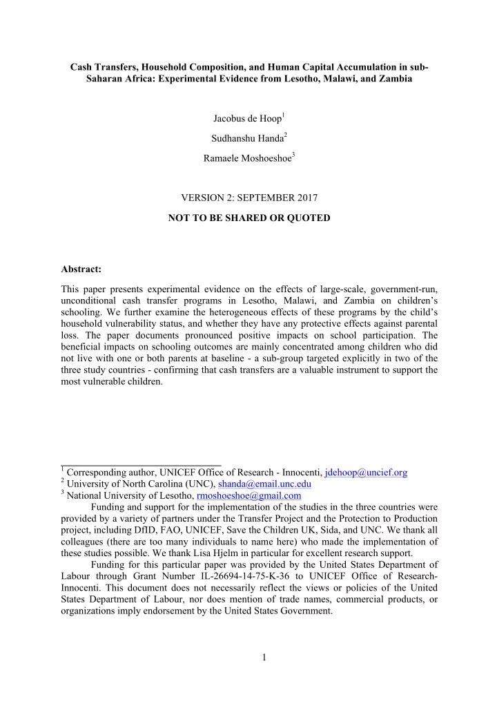
4.1 Overall and disaggregated impacts on schooling and child work Figure 1 shows school enrollment at baseline. The solid line shows the fraction of children enrolled in school (by age) in the control group, estimated by means of a local polynomial of order 1. The dashed line does the same for children in the treatment group. We

• bserve an inverse u-shaped pattern that peaks at the age of 13, when close to 90% of the

children in our sample are in school. At the age of 17, only about 60% of children in our sample are still enrolled. At baseline, school attendance in the treatment group closely resembles that of children in the control group. Figure 2 shows school enrollment at follow- up and indicates that the programs had a substantive effect on school enrollment. The school enrollment curve for the treatment group lies above that of the control group at all ages. However, the difference between the control and treatment group is somewhat larger for

• lder children.

Table 2 displays our estimated impacts on school participation based on regression specification (1). We find that school enrollment increased by over 6 percentage points if we rely on the pooled data (Panel A). Program impacts on regular school attendance are positive

13 The Lesotho and Malawi study designs comprise sampling weights. We retain these sampling

weights, but rescale them (i.e. multiply them by the inverse of the total value of the sampling weights for all children in Lesotho and Malawi respectively). In Zambia, all observations receive the same weight: the inverse

• f the number of children in the sample.

15 but not statistically significant in the pooled data. However, note that these estimates exclude Malawi, due to the different nature of the variable for regular school attendance for that

• country. If we turn to the effects disaggregated by country, displayed in Appendix Table A3,

we find no significant impacts on any of the three schooling outcomes in Lesotho, but strong and statistically significant increase in school enrollment and regular school attendance in both Malawi and Zambia. At 15 percentage points, the increase in regular school attendance in Malawi is particularly pronounced. Although the point estimates are positive for all three countries, we find no statistically significant increase in grade progression. Table 3 examines whether the estimated program effects on education outcomes are heterogeneous by age, gender, and baseline schooling status. Using gender as an example, we modify our regression specification to examine heterogeneous program effects as follows: (2) Yict = Ttc*Mic+ Ttc*Fic + dt* Mic + dt* Fic + di + εict where Mic is a dummy variable taking the value 1 if individual i is male and Fic is a dummy variable taking the value 1 if individual i is female. As shown in Panel A of Table 3, the program effects are most pronounced for older children (aged 11-17 at baseline, 13-19 at follow-up), who are in the age range at which children start dropping out of school. These children see their school enrollment and regular school attendance increase by respectively 9 and 6 percentage points vis-à-vis the control

• group. Impacts are comparable for boys and girls (Panel B) and for children who were in

school and children who were not (Panel C). The latter suggests that the programs both reduced school dropout and encouraged children who were previously not in school to enroll. As shown in Appendix tables A4A-A4C, these findings are reasonably consistent across the three countries. Importantly, we also find positive and significant impacts for two subgroups

• f children in Lesotho: older children and children who were in school at baseline.

16 4.2 Labor constraints Next, we examine how labor constraints affect program impacts on children’s

• education. As mentioned earlier, at baseline the household of the average child in our sample

consisted for about 30% of adults aged 18 to 65. In other terms, the average child came from a household with a dependency ratio of about 2.3 (this is a conservative measure of the dependency ratio, as a share of the adult household members may also be dependents, for instance due to illness and disability). As shown in the histogram displayed in figure 3, there is substantive variation in the fraction of adults across households and a sizeable fraction of children lives in a household without working age adults. Table 5 examines baseline correlations between our outcome variables and the fraction of adults in the household. We find a substantive positive correlation between all three schooling outcomes and the fraction of adults in the household. This implies that households with a larger fraction of adults have a larger capacity to carry out income generating activities. The associated higher level of household income is partly invested in children’s education, explaining better schooling outcomes in households with a higher fraction of adults. Table 6 examines whether program effects are heterogeneous by the fraction of adults in the household at baseline, based on the following regression specification: (3) Yict = Ttc+ Ttc*Fractionic + dt + dt* Fractionic + di + εict, where Fractionic is the fraction of adult members in the household of child i at baseline. We note that the coefficient of the treatment variable is positive and significant, indicating that cash transfer programs have a pronounced and positive impact on the school participation of children from households with no adults. The coefficient on the interaction term (Treatment *

17 Fraction of adults or Ttc*Fractionic) is negative and substantive (although not statistically significant), suggesting that improvements in schooling outcomes for children from households with a large fraction of adults are limited. These results suggest that, because households with fewer adults have lower income earning capacity, they under-invest in education at baseline. The receipt of the cash transfers opens up new opportunities to invest, in education and in productive household activities. Hence, children living in households with fewer adults are more likely to start attending school. 4.3 Protective effects We now proceed to examine whether receipt of the cash transfer program helps support the school attendance of children who do not live with - or lose - a parent. We first examine impacts on schooling outcomes for children who lived with their parents at baseline and children who did not, relying on regression specification (2). As shown in Table 7, Panel A, children were about five percentage points less likely to be enrolled in school and 3 percentage points less likely to attend school regularly when they did not live with their

• father. The effects of the cash transfer programs on school participation are located almost

exclusively in the latter group and essentially eliminate the gap in schooling outcomes between children who did and did not live with their father. The pattern is comparable when we look at absence of a child’s mother (Panel B) or absence of both of the child’s parents (Panel C). As mentioned also in the introduction, this finding supports explicit targeting of programs on orphans and vulnerable children.

18 Next, we examine how the death of a child’s father (mother) affects children and we examine whether receipt of cash transfers can reduce the detrimental effect of losing a father (mother).14 To do so, we estimate the following equation: (4) Yict = Ttc + Sitc + Ttc* Sitc + dt + di + εict Here, Sitc represents the binary indicator for experiencing the negative shock of losing a father (mother). In our analysis, we restrict our sample to children who were living with their father (mother) at baseline. Fitzsimons and Mesnard (2014) and de Janvry et al. (2006) rely on a similar specification to examine whether cash transfer programs can cushion the effect of economic shocks and keep children from entering work and dropping out of school in Colombia and Mexico. Using this regression specification, Table 8 examines how children’s schooling is affected when their father (Panel A) or mother (Panel B) dies in the period between the baseline and the follow-up interview. Panel C examines children who lived with at least one parent at baseline and shows how they are affected when both of their parents are deceased at follow-up. Obviously, identification comes from the relatively small number of children who lose a parent and hence statistical power in this analysis is low.15 Before turning to the regression results, we discuss two potential concerns related to this analysis. First, the death of a parent may not be a fully exogenous shock and may reflect -

• r be associated with - other determinants of children’s schooling outcomes. While we

recognize this concern, we believe that it is limited in our case. As in Fitzsimons and

14 When respondents indicate that they do not know whether a child’s father (mother) is alive, we treat

this as equivalent to death of the father (mother).

15 Identification of the estimated effect of losing a father comes from 100 out of 1,522 children in the

control group and 132 out of 1,340 children in the treatment group. Identification of the estimated effect of losing a mother comes from 160 out of 3,821 children in the control group and 184 out of 3,608 children in the treatment group. Identification of the estimated effect of losing both parents comes 90 out of 4,082 children in the control group and 136 out of 3,694 children in the treatment group

19 Mesnard (2014) and de Janvry et al. (2006), our difference-in-differences estimation strategy accounts for time-invariant differences between children who do and do not experience the death of a parent. Moreover, even if the death of a parent reflects a “deeper” shock or several simultaneous shocks to the household, this does not preclude us from capturing the protective effects of cash transfer programs when children face this scenario. Second, the probability of experiencing the death of a parent may be affected by the program, for instance because the program may allow households to procure medical treatment when household members fall ill. To examine this issue, column (1) of Table 6 relies on specification (1) to show how the program affected the probability of losing a

• parent. We note that the probability of losing a father (Panel A) and hence both parents

(Panel C) is somewhat higher in the treatment group than in the control group. However, because this effect is small in magnitude and that we have no intuitive explanation for its direction, we consider this to be a statistical artefact. Turning to the regression results, we note that the effect of losing a father appears to be limited and the point estimates are not statistically significant. (If anything, and somewhat puzzlingly, point estimates for death of a father on regular school attendance are positive and substantive.) Effects of losing a mother and losing both parents on school enrollment are of the expected sign and statistically significant. At 14 to 15 percentage points, the effect of losing both parents on school enrollment and regular school attendance is particularly

• pronounced. The ability of the cash transfer programs to dampen the contemporaneous effect
• f this shock on school participation appears to be limited. While the interaction effect

(Treatment*Both parents deceased i.e. Ttc* Sitc) is positive and substantive for school enrollment, it is not statistically significant. Moreover, the interaction effect is close to zero for regular school enrollment.

20

• 5. Discussion and conclusion

This paper examines the effects of scaled up unconditional cash transfer programs in three countries in Sub-Saharan Africa – Lesotho, Malawi, and Zambia – on children’s schooling outcomes. We find evidence of pronounced impacts on school participation, particularly among older children. Impacts on grade progression, however, are limited. We also show that these programs have stronger effects on the schooling outcomes of children who did not live with one of their parents or both of their parents at baseline. However, the programs do not immediately protect the school attendance of children when they lose a parent. How should we interpret the finding that (regular) school participation increased while impacts on grade progression are limited? One likely explanation is that the children who stay in school as a result of the program are a select group and may progress more slowly for instance because they face bigger personal obstacles to school attainment, are more intensively involved in productive activities, have lower (perceived or real) returns to education, etc. Limited school progression may also reflect a learning environment that does not adequately cater to the needs of this select group of children. The latter would suggest that, although cash transfers are a useful instrument to improve schooling outcomes, there are limits to what can be achieved with these programs in isolation. Improved grade progression and learning in school also depend on the availability and quality of schools and teachers. Why are we not able to replicate the finding in previous research (Fitzsimons and Mesnard, 2014) that cash transfers protect children when a parent (in their case father) leaves the household? A potential reason is that there are substantive contextual and cultural differences between the context of sub-Saharan Africa and that of Colombia. Exploring the role of these differences is beyond the scope of this paper. Another explanation could be that

21 a modest cash transfer is simply not sufficient to protect school participation when children go through a period of intensive re-adjustment after the death of a parent, particularly when they already reside in a vulnerable household with a high dependency ratio. Finally, we discuss some additional results from country-specific analyses, which help to further contextualize the cross-country findings presented in this paper. De Hoop et al. (2016a) examine the effects of Zambia’s MCTP on household productive activities. They document pronounced positive program “effects on beneficiary households’ crop production, livestock production and, to a lesser extent, non-agricultural entrepreneurial activities.” They show that all household members (adults, youths, and children) increased their engagement in these same activities, suggesting that households rely, at least partly, on children to exploit new investment opportunities, which may limit the effect of these programs on schooling.16 Relatedly, Sebastian et al. (2016) provide detailed evidence on the impacts of Lesotho’s cash transfer program, focusing particularly on agricultural households (about 86%

• f the overall sample). The authors examine whether program impacts on child activities

differ for female headed households and households headed by a married couple. Interestingly, older boys appear to benefit particularly when female-headed households receive the transfer, while older girls appear to benefit when households headed by a married couple receive the transfer. The authors provide multiple plausible explanations for these heterogeneous findings and, in accordance with the results presented in this paper conclude that “it is the household structure and constraints that determine these differentiated effects”.

16 They also examine impacts on underlying economic activities and household chores (data for these

underlying activities were not collected at baseline and hence not considered in the cohort analysis presented in this paper). This analysis confirms overall increased engagement in work and chores.

22 References Akresh, Richard, Damien de Walque, and Harounan Kazianga. 2013. “Cash Transfers and Child Schooling: Evidence from a Randomized Evaluation of the Role of Conditionality.” World Bank Policy Research Working Paper 6340. Baird, Sarah, Craig McIntosh, and Berk Özler. 2011. “Cash or Condition? Evidence from a Cash Transfer Experiment.” Quarterly Journal of Economics, 126 (4): 1709–53. Baird, Sarah, Francisco H. G. Ferreira, Berk Özler, and Michael Woolcock. 2014. “Conditional, Unconditional, and Everything in Between: A Systematic Review of the Effects of Cash Transfer Programmes on Schooling Outcomes.” Journal of Development Effectiveness, 6 (1): 1-43. Beegle, Kathleen, Joachim de Weerdt, and Stefan Dercon. 2010. “Orphanhood and Human Capital Destruction: Is there Persistence Into Adulthood?” Demography, 47 (1): 163- 180. Benhassine, Najy, Florencia Devoto, Esther Duflo, Pascaline Dupas, and Victor Poliquen.

• 2015. “Turning a Shove into a Nudge? A “Labeled Cash Transfer” for Education.”

American Econnomic Journal: Economic Policy, 7 (3), 86-125. Case, Anne, and Cally Ardington. 2006. “The Impact of Parental Death on School Outcomes: Longitudinal Evidence from South Africa.” Demograpgy, 43 (3): 401-420. Case, Anne, Christina Paxson, and Joseph Ableidinger. 2004. “Orphans in Africa: Parental Death, Poverty and School Enrolment.” Demography, 41 (3): 483-508. De Groot, Richard, Sudhanshu Handa, Michael Park, Robert Osei Darko, Isaac Osei-Akoto, Garima Bhalla, and Luigi Peter Ragno. 2015. “Heterogeneous Impacts of an Unconditional Cash Transfer Programme on Schooling: Evidence from the Ghana LEAP Programme.” UNICEF Office of Research – Innocenti Working Paper WP- 2015-10.

23 De Hoop, Jacobus, Sudhanshu Handa, and the Zambia MCP Evaluation Team. 2016a. “Cash Transfers, Household Production, and Household Members’ Activities: Evidence from an Experiment in Zambia.” Mimeo available on request. De Hoop, Jacobus, Sudhanshu Handa, and Susannah Zietz. 2016b. “Children’s Participation in Economic Activities and Household Chores in Malawi: A Qualitative Study on the Malawi Social Cash Transfer Programme.” Mimeo available on request. De Hoop, Jacobus and Furio C. Rosati. 2014. “Cash Transfers and Child Labor” World Bank Research Observer, 29 (2): 202-234. De Janvry, Alain, Frederico Finan, Elisabeth Sadoulet, and Renos Vakis. 2006. “Can Conditional Cash Transfer Programs Serve as Safety Nets in Keeping Children at School and from Working when Exposed to Shocks?” Journal of Development Economics, 79 (2): 349–73.Edmonds, Eric V. 2007. “Child Labour.” In Handbook of Development Economics, Volume 4, ed. T. P. Schultz, J. Strauss, 3607–709. Amsterdam: Elsevier Science. Edmonds, Eric V., and Norbert Schady. 2012. “Poverty Alleviation and Child Labor.” American Economic Journal: Economic Policy, 4 (4): 100–24. Evans, David, and Edward Miguel. 2007. “Orphans and Schooling in Africa: A Longitudinal Analysis.” Demography, 44 (1): 35-57. Fiszbein, Ariel, and Norbert Schady. 2009. Conditional Cash Transfers: Reducing Present and Future Poverty. The World Bank, Washington D.C. Fitzsimons, Emla, and Alice Mesnard. 2014. “Can Conditional Cash Transfers Compensate for a Father’s Absence?” World Bank Economic Review, 28 (3): 467-491. Gertler, Paul, David I. Levine, and Minnie Ames. 2004. “Schooling and Parental Death.” Review of Economics and Statistics, 86 (1): 211-225.

24 Gimenez, Lea, Shin-Yi Chou, Jin-Tan Liu, Jin-Long Liu. 2013. “Parental Loss and Children’s Well-being.” Journal of Human Resources, 48 (4): 1035-1071. Handa, Sudhanshu, Luisa Natali, David Seidenfeld, and Gelson Tembo. 2016a. “The Impact

• f Zambia’s Unconditional Child Grant on Schooling and Work: Results from a

Large-Scale Social Experiment.” Journal of Development Effectiveness, 8 (3): 346- 367. Handa, Sudhanshu, Luisa Natali, David Seidenfeld, Gelson Tembo, and Benjamin Davis.

• 2016b. “Can Unconditional Cash Transfers Lead to Sustainable Poverty Reduction?

Evidence from Two Government-Led Programmes in Zambia.” UNICEF Office of Research – Innocenti Working Paper WP-2016-21. Kenya CT-OVC Evaluation Team. 2012. “The Impact of Kenya’s Cash Transfer for Orphans and Vulnerable Children on Human Capital.” Journal of Development Effectiveness, 4 (1): 38-49. Ministry of Community Development, Mother, and Child Health. 2014. 24 Month Report for the Multiple Category Targeting Grant. Pellerano, Luca, Marta Moratti, Maja Jakobsen, Matej Bajgar, and Valentina Barca. 2014. “Child Grants Impact Evaluation: Follow-up Report.” Oxford Policy Management. Saavedra, Juan Esteban, and Sandra Garcia. 2012. “Impact of Conditional Cash Transfer Programs on Educational Outcomes in Developing Countries: A Meta Analysis.” Rand Working Paper WR-921-1. Sebastian, Ashwini, Ana Paula de la O Campos, Silvio Daidone, Benjamin Davis, Ousmane Niang, and Luca Pellerano. 2016. “Gender Differences in Child Investment Behaviour among Agricultural Households.” WIDER Working Paper 2016/107.

• UNC. Forthcoming. “Malawi Social Cash Transfer Programme: Endline Impact Evaluation

Report.” Carolina Population Center.

25 Figures Figure 1. Baseline school enrollment Figure 2. Follow-up school enrollment

.2 .4 .6 .8 1 5 6 7 8 9 10 11 12 13 14 15 16 17 Age at baseline Treatment Control .4 .6 .8 1 7 8 9 10 11 12 13 14 15 16 17 18 19 Age at endline Treatment Control

26 Figure 3. Histogram of baseline fraction of working age adults (18-65) in the household

2 4 6 Density .2 .4 .6 .8 Fraction of adults aged 18-65 at baseline

27 Tables

Table 1. Baseline balance (1) (2) (3) (4) (5) (6) Enrollment Regular attendance Grade progression Panel A: Outcome variables Treatment

• 0.0030

0.0061

• 0.0143

(0.0208) (0.0240) (0.0217) Mean in control 0,7376 0,601 0,4859 Observations 15,053 7,944 14,610 Panel B: Main background variables Age Male Fraction of adults Lives with father Lives with mother Lives with at least one parent Treatment

• 0.0952
• 0.0000

0.0092

• 0.0072
• 0.0204
• 0.0229

(0.0950) (0.0101) (0.0147) (0.0263) (0.0241) (0.0243) Mean in control 10,667 0,5196 0,3035 0,2498 0,585 0,6071 Observations 15,053 15,053 15,053 14,233 14,282 14,207 Cross-section OLS regression of baseline outcome variables and covariates on the indicator for treatment and a constant. All regressions are re-weighted to give each country equal weight in the regression. Sample restricted to children who were 5-17 at baseline and who were observed both at baseline and at follow-up. Regular attendance does not include Malawi, as we cannot construct a comparable indicator for that country. Clustered standard errors in parentheses. *** p<0.01, ** p<0.05, * p<0.1.

28 Table 2. Impacts on schooling outcomes (1) (2) (3) Enrollment Regular attendance Grade progression Impact 0.0632*** 0.0374 0.0224 (0.0199) (0.0258) (0.0166) Number of unique observations 15,053 7,944 14,610 Mean in control at follow-up 0.753 0.594 0.524 Impact estimates based on individual fixed effects regressions (Specification (1)). All regressions are re-weighted to give each country equal weight in the regression. Sample restricted to children who were 5-17 at baseline and who were observed both at baseline and at follow-up. Regular attendance takes the value 1 if children did not miss any days of school in the 30 days (Lesotho) and the week (Zambia) prior to the interview. Regular attendance does not include Malawi, as we cannot construct a comparable indicator for that country. Grade progression refers to highest grade completed divided by age appropriate grade. Clustered standard errors in parentheses. *** p<0.01, ** p<0.05, * p<0.1.

29 Table 3. Heterogeneous impacts on schooling outcomes (1) (2) (3) Enrollment Regular attendance Grade progression Panel A: heterogeneity by age (i) Impact on children aged ≤10 at baseline 0.0258

• 0.0009

0.0440 (0.0220) (0.0309) (0.0319) (ii) Impact on children aged >10 at baseline 0.0879*** 0.0550** 0.0024 (0.0195) (0.0278) (0.0077) Number of unique observations 15,053 7,944 14,610 P-value for F-test: (i)=(ii) 0.00754 0.0900 0.166 Mean in control at follow-up ≤10 0.865 0.679 0.485 Mean in control at follow-up >10 0.648 0.525 0.558 Panel B: heterogeneity by gender (i) Impact on boys 0.0721*** 0.0450 0.0392* (0.0232) (0.0293) (0.0215) (ii) Impact on girls 0.0546** 0.0261 0.0062 (0.0213) (0.0303) (0.0170) Number of unique observations 15,038 7,931 14,597 P-value for F-test: (i)=(ii) 0.389 0.522 0.107 Mean in control at follow-up boys 0.736 0.570 0.501 Mean in control at follow-up girls 0.770 0.623 0.549 Panel C: heterogeneity by baseline schooling status (i) Impact on children in school at baseline 0.0599*** 0.0386 0.0221 (0.0134) (0.0344) (0.0202) (ii) Impact on children not in school at baseline 0.0635** 0.0278 0.0151 (0.0256) (0.0303) (0.0312) Number of unique observations 15,053 7,944 14,610 P-value for F-test: (i)=(ii) 0.879 0.783 0.846 Mean in control at follow-up boys 0.820 0.660 0.597 Mean in control at follow-up girls 0.564 0.396 0.314 Impact estimates based on individual fixed effects regressions (Specification (2)). All regressions are re-weighted to give each country equal weight in the regression. Sample restricted to children who were 5-17 at baseline and who were observed both at baseline and at follow-up. Regular attendance takes the value 1 if children did not miss any days of school in the 30 days (Lesotho) and the week (Zambia) prior to the interview. Regular attendance does not include Malawi, as we cannot construct a comparable indicator for that country. Grade progression refers to highest grade completed divided by age appropriate grade. Clustered standard errors in parentheses. *** p<0.01, ** p<0.05, * p<0.1.

30

Table 4. Correlation with fraction of adults aged 18-65 in the household (1) (2) (3) Enrollment Regular attendance Grade progression Fraction of adults 0.2284*** 0.1173** 0.1930*** (0.0299) (0.0467) (0.0514) Intercept 0,6657 0,5636 0,4204 Number of unique observations 15,053 7,944 14,610 Cross-section OLS regression of baseline outcome variables on the fraction of working age adults (aged 18-65) at baseline). All regressions are re-weighted to give each country equal weight in the regression. Sample restricted to children who were 5-17 at baseline and who were observed both at baseline and at follow-up. Regular attendance takes the value 1 if children did not miss any days of school in the 30 days (Lesotho) and the week (Zambia) prior to the

• interview. Regular attendance does not include Malawi, as we cannot construct

a comparable indicator for that country. Grade progression refers to highest grade completed divided by age appropriate grade. Clustered standard errors in

• parentheses. *** p<0.01, ** p<0.05, * p<0.1.

31 Table 5. Heterogeneous impacts by fraction of adult household members at baseline (1) (2) (3) Enrollment Regular attendance Grade progression Treatment 0.0944*** 0.0608 0.0188 (0.0260) (0.0432) (0.0312) Treatment * Fraction of adults

• 0.0966
• 0.0680

0.0094 (0.0605) (0.1133) (0.1019) Number of unique observations 15,053 7,944 14,610 Impact estimates based on individual fixed effects regressions (Specification (3)). All regressions are re-weighted to give each country equal weight in the regression. Sample restricted to children who were 5-17 at baseline and who were observed both at baseline and at follow-up. Regular attendance takes the value 1 if children did not miss any days of school in the 30 days (Lesotho) and the week (Zambia) prior to the interview. Regular attendance does not include Malawi, as we cannot construct a comparable indicator for that

• country. Grade progression refers to highest grade completed divided by age appropriate
• grade. Clustered standard errors in parentheses. *** p<0.01, ** p<0.05, * p<0.1.

32 Table 6. Heterogeneous impacts by presence of parents at baseline (1) (2) (3) Enrollment Regular attendance Grade progression Panel A: (i) Lived with father at baseline 0.0159 0.0048 0.0174 (0.0264) (0.0463) (0.0208) (ii) Did not live with father at baseline 0.0784*** 0.0497* 0.0250 (0.0212) (0.0269) (0.0192) Number of unique observations 14,945 7,845 14,507 P-value for F-test: (i)=(ii) 0.0153 0.349 0.755 Mean in control at follow-up, lived with father 0.789 0.615 0.545 Mean in control at follow-up, did not live with father 0.742 0.587 0.518 Panel B: (i) Lived with mother at baseline 0.0364*

• 0.0087

0.0299 (0.0220) (0.0303) (0.0208) (ii) Did not live with mother at baseline 0.1022*** 0.1025*** 0.0156 (0.0231) (0.0356) (0.0207) Number of unique observations 14,987 7,880 14,549 P-value for F-test: (i)=(ii) 0.00236 0.00657 0.569 Mean in control at follow-up, lived with mother 0.771 0.612 0.520 Mean in control at follow-up, did not live with mothe 0.728 0.568 0.529 Panel C: (i) Lived with at least one parent at baseline 0.0370*

• 0.0043

0.0311 (0.0221) (0.0291) (0.0203) (ii) Did not live with a parent at baseline 0.1044*** 0.1040*** 0.0156 (0.0238) (0.0365) (0.0212) Number of unique observations 14,925 7,825 14,488 P-value for F-test: (i)=(ii) 0.00297 0.00744 0.533 Mean in control at follow-up, lived with mother 0.771 0.612 0.523 Mean in control at follow-up, did not live with mothe 0.727 0.566 0.525 Impact estimates based on individual fixed effects regressions (Specification (2)). All regressions are re-weighted to give each country equal weight in the regression. Sample restricted to children who were 5-17 at baseline and who were observed both at baseline and at follow-up. Regular attendance takes the value 1 if children did not miss any days of school in the 30 days (Lesotho) and the week (Zambia) prior to the interview. Regular attendance does not include Malawi, as we cannot construct a comparable indicator for that country. Grade progression refers to highest grade completed divided by age appropriate grade. Clustered standard errors in parentheses. *** p<0.01, ** p<0.05, * p<0.1.

33

Table 7. Protective effects when losing a parent (1) (2) (3) (4) Occurrence

• f death

Enrollment Regular attendance Grade progression Panel A (sample: father lived in HH at baseline): Treatment 0.0257* 0.0166 0.0119 0.0227 (0.0153) (0.0265) (0.0532) (0.0252) Father deceased 0.0059 0.1287 0.0428 (0.0620) (0.1155) (0.0615) Treatment*Father deceased 0.0067

• 0.0545
• 0.0577

(0.0724) (0.1489) (0.0739) Number of unique observations 2,862 2,862 1,570 2,698 Panel B (sample: mother lived in HH at baseline): Treatment 0.0118 0.0331

• 0.0055

0.0322 (0.0089) (0.0217) (0.0342) (0.0244) Mother deceased

• 0.0741*
• 0.0549

0.0250 (0.0400) (0.0544) (0.0362) Treatment*Mother deceased 0.0175

• 0.0540
• 0.0145

(0.0538) (0.0779) (0.0451) Number of unique observations 7,589 7,589 3,812 7,307 Panel C (sample: at least one parent in HH at baseline): Treatment 0.0117* 0.0336 0.0014 0.0325 (0.0068) (0.0213) (0.0318) (0.0243) Both parents deceased

• 0.1524***
• 0.1405**

0.0164 (0.0439) (0.0607) (0.0448) Treatment*Both parents deceased 0.0901 0.0076

• 0.0224

(0.0606) (0.0866) (0.0531) Number of unique observations 7,776 7,776 3,946 7,484 Program impact on occurence of shock (column (1)) estimated based on individual fixed effects regressions (Specification (1)). Remaining impact estimates (columns (2)-(4)) based on individual fixed effects regressions (Specification (4)). All regressions are re-weighted to give each country equal weight in the regression. Sample restricted to children who were 5-17 at baseline and who were observed both at baseline and at follow-up. Regular attendance takes the value 1 if children did not miss any days of school in the 30 days (Lesotho) and the week (Zambia) prior to the interview. Regular attendance does not include Malawi, as we cannot construct a comparable indicator for that country. Grade progression refers to highest grade completed divided by age appropriate grade. Clustered standard errors in parentheses. *** p<0.01, ** p<0.05, * p<0.1.

34 Appendix 1. Attrition Appendix Table A1 examines whether sample attrition differs for our treatment and control group. Column (1) focuses on the pooled sample of 17,513 children and shows the results of regressing the indicator variable for child being observed at follow-up on a constant and the indicator for treatment. As in the remainder of the analysis presented in this paper,

• bservations are re-weighted according to the number of observations per country (see the

section on regression specification) and standard errors are clustered at the level of treatment

• assignment. Columns (2) – (4) contain the same analysis, but at the country level.

There is no evidence of differential attrition in the pooled data. The treatment coefficient is small and not statistically significant. However, we note that there is e differential attrition at the country level: children from treatment households are more likely to be observed at follow-up in Lesotho and less likely to be observed at follow-up in Malawi and Zambia. In aggregate, these attrition patterns cancel out. Table A1. Attrition (1) (2) (3) (4) Pooled Lesotho Malawi Zambia Treatment 0.0038 0.0707***

• 0.0315
• 0.0307**

(0.0114) (0.0196) (0.0194) (0.0147) Constant 0.8597*** 0.8433*** 0.8572*** 0.8786*** (0.0078) (0.0161) (0.0144) (0.0094) Observations 17,513 2,951 7,888 6,674 Cross-section OLS regression of indicator variable for child observed at follow-up on the indicator for treatment and a constant. All regressions are re-weighted to give each country equal weight in the regression. Sample restricted to children who were 5-17 at baseline. Clustered standard errors in parentheses. *** p<0.01, ** p<0.05, * p<0.1.

35 Appendix 2. Country-specific results

Table A2. Baseline balance by country (1) (2) (3) (4) (5) (6) Enrollment Regular attendance Grade progression Panel A: Lesotho Treatment 0.0344* 0.0453

• 0.0183

(0.0176) (0.0364) (0.0373) Mean in control 0,862 0,6539 0,6399 Observations 2,567 2,399 2,204 Panel B: Malawi Treatment

• 0.0212
• 0.0210

0.0011 (0.0317) (0.0359) (0.0292) Mean in control 0,6972 0,6054 0,448 Observations 6,727 6,727 6,727 Panel C: Zambia Treatment

• 0.0498**
• 0.0391*
• 0.0499**

(0.0223) (0.0235) (0.0224) Mean in control 0,6654 0,5525 0,4036 Observations 5,759 5,545 5,679 Age Male Fraction of adults Lives with father Lives with mother Lives with at least one parent Panel D: Lesotho Treatment

• 0.1627

0.0159 0.0089

• 0.0048

0.0077

• 0.0048

(0.1570) (0.0237) (0.0126) (0.0486) (0.0397) (0.0385) Mean in control 10,8058 0,5047 0,4039 0,3824 0,6122 0,6582 Observations 2,567 2,567 2,567 2,232 2,241 2,219 Panel E: Malawi Treatment 0.0494 0.0084

• 0.0014
• 0.0289
• 0.0452
• 0.0446

(0.1148) (0.0113) (0.0119) (0.0333) (0.0442) (0.0443) Mean in control 10,2187 0,508 0,2257 0,1989 0,596 0,6029 Observations 6,727 6,727 6,727 6,707 6,707 6,707 Panel F: Zambia Treatment

• 0.2321*
• 0.0241*
• 0.0048
• 0.0154
• 0.0275
• 0.0283

(0.1296) (0.0129) (0.0110) (0.0317) (0.0399) (0.0403) Mean in control 11,0133 0,5457 0,2933 0,1924 0,549 0,5676 Observations 5,759 5,759 5,759 5,294 5,334 5,281 Cross-section OLS regression of baseline outcome variables and covariates on the indicator for treatment and a constant. All regressions are re-weighted to give each country equal weight in the regression. Sample restricted to children who were 5-17 at baseline and who were observed both at baseline and at follow-up. Regular attendance takes the value 1 if children did not miss any days of school in the 30 days (Lesotho) and the week (Zambia) prior to the interview. Regular attendance takes the value 1 in Malawi if the child did not miss two consecutive weeks of instruction in the past 12

• months. Grade progression refers to highest grade completed divided by age appropriate grade. Clustered standard errors

in parentheses. *** p<0.01, ** p<0.05, * p<0.1.

36 Table A3. Impacts on schooling outcomes by country (1) (2) (3) Enrollment Regular attendance Grade progression Panel A: Lesotho: Impact 0.0245 0.0180 0.0298 (0.0224) (0.0410) (0.0328) Number of unique observations 2,567 2,399 2,204 Mean in control at follow-up 0.824 0.699 0.699 Panel B: Malawi: Impact 0.0915*** 0.1459*** 0.0259 (0.0279) (0.0253) (0.0265) Number of unique observations 6,727 6,727 6,727 Mean in control at follow-up 0.790 0.697 0.434 Panel C: Zambia: Impact 0.0963*** 0.0533* 0.0047 (0.0207) (0.0312) (0.0133) Number of unique observations 5,759 5,545 5,679 Mean in control at follow-up 0.653 0.511 0.489 Impact estimates based on individual fixed effects regressions (Specification (1)). Sample restricted to children who were 5-17 at baseline and who were observed both at baseline and at follow-up. Regular attendance takes the value 1 if children did not miss any days of school in the 30 days (Lesotho) and the week (Zambia) prior to the

• interview. In Malawi, regular attendance takes the value 1 if the child did not miss two

consecutive weeks of instruction in the past 12 months. Grade progression refers to highest grade completed divided by age appropriate grade. Clustered standard errors in

• parentheses. *** p<0.01, ** p<0.05, * p<0.1.

37 Table A4A. Heterogeneous impacts on schooling outcomes by age (1) (2) (3) Enrollment Regular attendance Grade progression Panel A: Lesotho (i) Impact on children aged ≤10 at baseline

• 0.0596**
• 0.0286

0.0729 (0.0241) (0.0469) (0.0772) (ii) Impact on children aged >10 at baseline 0.0810** 0.0412

• 0.0064

(0.0315) (0.0433) (0.0099) Number of unique observations 2,567 2,399 2,204 P-value for F-test: (i)=(ii) 0.000648 0.161 0.294 Mean in control at follow-up ≤10 0.991 0.840 0.745 Mean in control at follow-up >10 0.686 0.588 0.673 Panel B: Malawi (i) Impact on children aged ≤10 at baseline 0.0910** 0.1372*** 0.0381 (0.0340) (0.0314) (0.0393) (ii) Impact on children aged >10 at baseline 0.0922*** 0.1566*** 0.0110 (0.0250) (0.0264) (0.0152) Number of unique observations 6,727 6,727 6,727 P-value for F-test: (i)=(ii) 0.970 0.556 0.406 Mean in control at follow-up ≤10 0.876 0.785 0.422 Mean in control at follow-up >10 0.686 0.589 0.448 Panel C: Zambia (i) Impact on children aged ≤10 at baseline 0.0661** 0.0230

• 0.0003

(0.0260) (0.0394) (0.0257) (ii) Impact on children aged >10 at baseline 0.1017*** 0.0655* 0.0057 (0.0263) (0.0354) (0.0121) Number of unique observations 5,759 5,545 5,679 P-value for F-test: (i)=(ii) 0.328 0.334 0.834 Mean in control at follow-up ≤10 0.727 0.552 0.404 Mean in control at follow-up >10 0.595 0.477 0.556 Impact estimates based on individual fixed effects regressions (Specification (2)). Sample restricted to children who were 5-17 at baseline and who were observed both at baseline and at follow-up. Regular attendance takes the value 1 if children did not miss any days of school in the 30 days (Lesotho) and the week (Zambia) prior to the interview. In Malawi, regular attendance takes the value 1 if the child did not miss two consecutive weeks of instruction in the past 12 months. Grade progression refers to highest grade completed divided by age appropriate grade. Clustered standard errors in parentheses. *** p<0.01, ** p<0.05, * p<0.1.

38 Table A4B. Heterogeneous impacts on schooling outcomes by gender (1) (2) (3) Enrollment Regular attendance Grade progression Panel A: Lesotho (i) Impact on boys 0.0445 0.0332 0.0907* (0.0291) (0.0480) (0.0538) (ii) Impact on girls 0.0073

• 0.0031
• 0.0298

(0.0316) (0.0471) (0.0237) Number of unique observations 2,558 2,391 2,197 P-value for F-test: (i)=(ii) 0.372 0.446 0.0233 Mean in control at follow-up boys 0.792 0.668 0.641 Mean in control at follow-up girls 0.855 0.739 0.770 Panel B: Malawi (i) Impact on boys 0.0916*** 0.1639*** 0.0264 (0.0302) (0.0312) (0.0245) (ii) Impact on girls 0.0909*** 0.1267*** 0.0254 (0.0315) (0.0290) (0.0324) Number of unique observations 6,727 6,727 6,727 P-value for F-test: (i)=(ii) 0.979 0.262 0.963 Mean in control at follow-up boys 0.797 0.689 0.421 Mean in control at follow-up girls 0.783 0.705 0.447 Panel C: Zambia (i) Impact on boys 0.1073*** 0.0532 0.0034 (0.0245) (0.0347) (0.0182) (ii) Impact on girls 0.0843*** 0.0533 0.0065 (0.0279) (0.0372) (0.0176) Number of unique observations 5,753 5,540 5,673 P-value for F-test: (i)=(ii) 0.476 0.998 0.898 Mean in control at follow-up boys 0.648 0.508 0.490 Mean in control at follow-up girls 0.659 0.511 0.488 Impact estimates based on individual fixed effects regressions (Specification (2)). Sample restricted to children who were 5-17 at baseline and who were observed both at baseline and at follow-up. Regular attendance takes the value 1 if children did not miss any days of school in the 30 days (Lesotho) and the week (Zambia) prior to the interview. In Malawi, regular attendance takes the value 1 if the child did not miss two consecutive weeks of instruction in the past 12 months. Grade progression refers to highest grade completed divided by age appropriate grade. Clustered standard errors in parentheses. *** p<0.01, ** p<0.05, * p<0.1.

39 Table A4C. Heterogeneous impacts on schooling outcomes by baseline schooling status (1) (2) (3) Enrollment Regular attendance Grade progression Panel A: Lesotho (i) Impact on children in school at baseline 0.0605*** 0.0401 0.0110 (0.0207) (0.0440) (0.0216) (ii) Impact on children not in school at baseline

• 0.0401
• 0.0177

0.2338 (0.0618) (0.0712) (0.2401) Number of unique observations 2,567 2,399 2,204 P-value for F-test: (i)=(ii) 0.118 0.458 0.349 Mean in control at follow-up boys 0.859 0.738 0.727 Mean in control at follow-up girls 0.600 0.472 0.550 Panel B: Malawi (i) Impact on children in school at baseline 0.0584*** 0.1170*** 0.0170 (0.0159) (0.0226) (0.0398) (ii) Impact on children not in school at baseline 0.1099*** 0.1648*** 0.0262 (0.0270) (0.0307) (0.0238) Number of unique observations 6,727 6,727 6,727 P-value for F-test: (i)=(ii) 0.0346 0.239 0.835 Mean in control at follow-up boys 0.859 0.769 0.502 Mean in control at follow-up girls 0.631 0.532 0.278 Panel C: Zambia (i) Impact on children in school at baseline 0.0507*** 0.0077 0.0230 (0.0186) (0.0362) (0.0172) (ii) Impact on children not in school at baseline 0.0704*** 0.0476

• 0.0435*

(0.0266) (0.0318) (0.0230) Number of unique observations 5,759 5,545 5,679 P-value for F-test: (i)=(ii) 0.491 0.267 0.0341 Mean in control at follow-up boys 0.736 0.581 0.584 Mean in control at follow-up girls 0.488 0.366 0.300 Impact estimates based on individual fixed effects regressions (Specification (2)). Sample restricted to children who were 5-17 at baseline and who were observed both at baseline and at follow-up. Regular attendance takes the value 1 if children did not miss any days of school in the 30 days (Lesotho) and the week (Zambia) prior to the interview. In Malawi, regular attendance takes the value 1 if the child did not miss two consecutive weeks of instruction in the past 12 months. Grade progression refers to highest grade completed divided by age appropriate grade. Clustered standard errors in parentheses. *** p<0.01, ** p<0.05, * p<0.1.

40

Table A6. Correlation with fraction of adults aged 18-65 in the household (1) (2) (3) Enrollment Regular attendance Grade progression Panel A: Lesotho Fraction of adults

• 0.0013
• 0.1229
• 0.0563

(0.0370) (0.0765) (0.1166) Intercept 0,8812 0,7278 0,6529 Number of unique observations 2,567 2,399 2,204 Panel B: Malawi Fraction of adults

• 0.0647
• 0.0321
• 0.0902

(0.0506) (0.0621) (0.0539) Intercept 0,7017 0,6027 0,4688 Number of unique observations 6,727 6,727 6,727 Panel C: Zambia Fraction of adults 0.1089** 0.0753 0.1429*** (0.0436) (0.0513) (0.0402) Intercept 0,6087 0,5109 0,337 Number of unique observations 5,759 5,545 5,679 Cross-section OLS regression of baseline outcome variables on the fraction of working age adults (aged 18-65) at baseline). Sample restricted to children who were 5-17 at baseline and who were observed both at baseline and at follow-

• up. Regular attendance takes the value 1 if children did not miss any days of

school in the 30 days (Lesotho) and the week (Zambia) prior to the interview. In Malawi, regular attendance takes the value 1 if the child did not miss two consecutive weeks of instruction in the past 12 months. Grade progression refers to highest grade completed divided by age appropriate grade. Clustered standard errors in parentheses. *** p<0.01, ** p<0.05, * p<0.1.

41 Table A7. Heterogeneous impacts by fraction of adult household members at baseline (1) (2) (3) Enrollment Regular attendance Grade progression Panel A: Lesotho Treatment

• 0.0042

0.0334

• 0.0476

(0.0463) (0.0762) (0.0718) Treatment * Fraction of adults 0.0699

• 0.0396

0.1898 (0.1106) (0.1691) (0.2210) Number of unique observations 2,567 2,399 2,204 Panel B: Malawi Treatment 0.1009*** 0.1526*** 0.0488 (0.0291) (0.0287) (0.0358) Treatment * Fraction of adults

• 0.0413
• 0.0290
• 0.1008

(0.1116) (0.1170) (0.1167) Number of unique observations 6,727 6,727 6,727 Panel C: Zambia Treatment 0.1259*** 0.0710 0.0207 (0.0395) (0.0522) (0.0271) Treatment * Fraction of adults

• 0.1043
• 0.0631
• 0.0558

(0.1080) (0.1432) (0.0738) Number of unique observations 5,759 5,545 5,679 Impact estimates based on individual fixed effects regressions (Specification (3)). Sample restricted to children who were 5-17 at baseline and who were observed both at baseline and at follow-up. Regular attendance takes the value 1 if children did not miss any days of school in the 30 days (Lesotho) and the week (Zambia) prior to the interview. In Malawi, regular attendance takes the value 1 if the child did not miss two consecutive weeks of instruction in the past 12 months. Grade progression refers to highest grade completed divided by age appropriate grade. Clustered standard errors in parentheses. *** p<0.01, ** p<0.05, * p<0.1.

42 Table A8A. Heterogeneous impacts by presence of father at baseline (1) (2) (3) Enrollment Regular attendance Grade progression Panel A: Lesotho (i) Lived with father at baseline 0.0047

• 0.0027

0.0649** (0.0297) (0.0636) (0.0327) (ii) Did not live with father at baseline 0.0356 0.0280 0.0107 (0.0307) (0.0450) (0.0457) Number of unique observations 2,531 2,366 2,172 P-value for F-test: (i)=(ii) 0.463 0.653 0.291 Mean in control at follow-up, lived with father 0.851 0.706 0.704 Mean in control at follow-up, did not live with father 0.813 0.701 0.708 Panel B: Malawi (i) Lived with father at baseline 0.0396 0.1007* 0.0041 (0.0491) (0.0514) (0.0372) (ii) Did not live with father at baseline 0.1045*** 0.1579*** 0.0321 (0.0293) (0.0259) (0.0286) Number of unique observations 6,727 6,727 6,727 P-value for F-test: (i)=(ii) 0.190 0.264 0.503 Mean in control at follow-up, lived with father 0.824 0.745 0.423 Mean in control at follow-up, did not live with father 0.782 0.685 0.437 Panel C: Zambia (i) Lived with father at baseline 0.0646* 0.0132

• 0.0603**

(0.0366) (0.0552) (0.0279) (ii) Did not live with father at baseline 0.1026*** 0.0636* 0.0208 (0.0224) (0.0330) (0.0138) Number of unique observations 5,687 5,479 5,608 P-value for F-test: (i)=(ii) 0.345 0.381 0.00663 Mean in control at follow-up, lived with father 0.686 0.542 0.490 Mean in control at follow-up, did not live with father 0.646 0.503 0.490 Impact estimates based on individual fixed effects regressions (Specification (2)). Sample restricted to children who were 5-17 at baseline and who were observed both at baseline and at follow-up. Regular attendance takes the value 1 if children did not miss any days of school in the 30 days (Lesotho) and the week (Zambia) prior to the interview. In Malawi, regular attendance takes the value 1 if the child did not miss two consecutive weeks of instruction in the past 12 months. Grade progression refers to highest grade completed divided by age appropriate grade. Clustered standard errors in parentheses. *** p<0.01, ** p<0.05, * p<0.1.

43 Table A8B. Heterogeneous impacts by presence of mother at baseline (1) (2) (3) Enrollment Regular attendance Grade progression Panel A: Lesotho (i) Lived with mother at baseline 0.0094

• 0.0311

0.0860* (0.0232) (0.0468) (0.0481) (ii) Did not live with mother at baseline 0.0460 0.0943

• 0.0504*

(0.0386) (0.0610) (0.0286) Number of unique observations 2,543 2,376 2,184 P-value for F-test: (i)=(ii) 0.382 0.0679 0.0111 Mean in control at follow-up, lived with mother 0.839 0.713 0.701 Mean in control at follow-up, did not live with mothe 0.805 0.689 0.713 Panel B: Malawi (i) Lived with mother at baseline 0.0853*** 0.1403*** 0.0257 (0.0304) (0.0284) (0.0248) (ii) Did not live with mother at baseline 0.1075*** 0.1596*** 0.0326 (0.0309) (0.0305) (0.0373) Number of unique observations 6,727 6,727 6,727 P-value for F-test: (i)=(ii) 0.411 0.528 0.844 Mean in control at follow-up, lived with mother 0.802 0.702 0.426 Mean in control at follow-up, did not live with mothe 0.774 0.690 0.445 Panel C: Zambia (i) Lived with mother at baseline 0.0489** 0.0104

• 0.0305*

(0.0245) (0.0358) (0.0177) (ii) Did not live with mother at baseline 0.1544*** 0.1083** 0.0449** (0.0298) (0.0414) (0.0211) Number of unique observations 5,717 5,504 5,638 P-value for F-test: (i)=(ii) 0.00405 0.0333 0.00860 Mean in control at follow-up, lived with mother 0.669 0.523 0.483 Mean in control at follow-up, did not live with mothe 0.634 0.491 0.498 Impact estimates based on individual fixed effects regressions (Specification (2)). Sample restricted to children who were 5-17 at baseline and who were observed both at baseline and at follow-up. Regular attendance takes the value 1 if children did not miss any days of school in the 30 days (Lesotho) and the week (Zambia) prior to the interview. In Malawi, regular attendance takes the value 1 if the child did not miss two consecutive weeks of instruction in the past 12 months. Grade progression refers to highest grade completed divided by age appropriate grade. Clustered standard errors in parentheses. *** p<0.01, ** p<0.05, * p<0.1.

44 Table A8C. Heterogeneous impacts by presence of any parents at baseline (1) (2) (3) Enrollment Regular attendance Grade progression Panel A: Lesotho (i) Lived with at least one parent at baseline 0.0111

• 0.0248

0.0840* (0.0228) (0.0448) (0.0456) (ii) Did not live with a parent at baseline 0.0489 0.0975

• 0.0593**

(0.0440) (0.0647) (0.0293) Number of unique observations 2,522 2,357 2,164 P-value for F-test: (i)=(ii) 0.427 0.0796 0.00474 Mean in control at follow-up, lived with a parent 0.837 0.711 0.701 Mean in control at follow-up, did not live a parent 0.804 0.688 0.717 Panel B: Malawi (i) Lived with at least one parent at baseline 0.0846** 0.1384*** 0.0233 (0.0308) (0.0283) (0.0253) (ii) Did not live with a parent at baseline 0.1081*** 0.1620*** 0.0359 (0.0314) (0.0314) (0.0378) Number of unique observations 6,727 6,727 6,727 P-value for F-test: (i)=(ii) 0.416 0.457 0.734 Mean in control at follow-up, lived with a parent 0.801 0.701 0.427 Mean in control at follow-up, did not live a parent 0.774 0.691 0.444 Panel C: Zambia (i) Lived with at least one parent at baseline 0.0502** 0.0148

• 0.0236

(0.0247) (0.0345) (0.0178) (ii) Did not live with a parent at baseline 0.1560*** 0.1075** 0.0434** (0.0300) (0.0417) (0.0206) Number of unique observations 5,676 5,468 5,597 P-value for F-test: (i)=(ii) 0.00475 0.0396 0.0181 Mean in control at follow-up, lived with a parent 0.670 0.525 0.484 Mean in control at follow-up, did not live a parent 0.631 0.489 0.498 Impact estimates based on individual fixed effects regressions (Specification (2)). Sample restricted to children who were 5-17 at baseline and who were observed both at baseline and at follow-up. Regular attendance takes the value 1 if children did not miss any days of school in the 30 days (Lesotho) and the week (Zambia) prior to the interview. In Malawi, regular attendance takes the value 1 if the child did not miss two consecutive weeks of instruction in the past 12 months. Grade progression refers to highest grade completed divided by age appropriate grade. Clustered standard errors in parentheses. *** p<0.01, ** p<0.05, * p<0.1.

45 Table A10A. Protective effects when losing a father by country (1) (2) (3) (4) Occurrence

• f death

Enrollment Regular attendance Grade progression Panel A, Lesotho: Treatment 0,0207 0.0230 0.0049 0.0780* (0.0180) (0.0289) (0.0712) (0.0414) Father deceased 0.1401 0.3255 0.1227 (0.1302) (0.2000) (0.0953) Treatment*Father deceased

• 0.2051
• 0.2848
• 0.1250

(0.1355) (0.2655) (0.1211) Number of unique observations 755 755 700 614 Panel B, Malawi: Treatment 0.0263 0.0177 0.0833

• 0.0027

(0.0279) (0.0481) (0.0510) (0.0423) Father deceased 0.0025 0.0261

• 0.0659

(0.1085) (0.1016) (0.0744) Treatment*Father deceased 0.0509 0.0257 0.0869 (0.1273) (0.1171) (0.1049) Number of unique observations 1,206 1,206 1,206 1,206 Panel C, Zambia: Treatment 0.0507 0.0562 0.0193

• 0.0652**

(0.0356) (0.0394) (0.0656) (0.0323) Father deceased

• 0.1199

0.0707 0.0612 (0.0836) (0.1274) (0.1040) Treatment*Father deceased 0.1073 0.0551

• 0.0829

(0.1066) (0.1622) (0.1194) Number of unique observations 901 901 870 878 Program impact on occurence of shock (column (1)) estimated based on individual fixed effects regressions (Specification (1)). Remaining impact estimates (columns (2)-(4)) based on individual fixed effects regressions (Specification (4)). Sample restricted to children who were 5-17 at baseline and who were observed both at baseline and at follow-up. Regular attendance takes the value 1 if children did not miss any days of school in the 30 days (Lesotho) and the week (Zambia) prior to the

• interview. In Malawi, regular attendance takes the value 1 if the child did not miss

two consecutive weeks of instruction in the past 12 months. Grade progression refers to highest grade completed divided by age appropriate grade. Clustered standard errors in parentheses. *** p<0.01, ** p<0.05, * p<0.1.

46

Table A10B. Protective effects when losing a mother by country (1) (2) (3) (4) Occurrence

• f death

Enrollment Regular attendance Grade progression Panel A, Lesotho: Treatment 0.0180 0.0036

• 0.0337

0.0985 (0.0183) (0.0231) (0.0533) (0.0594) Mother deceased

• 0.0588
• 0.1187*
• 0.0250

(0.0554) (0.0711) (0.0595) Treatment*Mother deceased

• 0.0372
• 0.0089
• 0.0077

(0.0765) (0.1133) (0.0780) Number of unique observations 1,352 1,352 1,260 1,112 Panel B, Malawi: Treatment

• 0.0055

0.0752** 0.1309*** 0.0276 (0.0086) (0.0313) (0.0301) (0.0266) Mother deceased

• 0.1281**
• 0.0535

0.0324 (0.0583) (0.0656) (0.0858) Treatment*Mother deceased 0.1237 0.0675

• 0.0181

(0.0825) (0.0859) (0.0988) Number of unique observations 3,601 3,601 3,601 3,601 Panel C, Zambia: Treatment 0.0212 0.0504* 0.0203

• 0.0388*

(0.0145) (0.0264) (0.0389) (0.0205) Mother deceased

• 0.0310

0.0059 0.0385 (0.0803) (0.0763) (0.0421) Treatment*Mother deceased 0.0410

• 0.0915
• 0.0142

(0.1003) (0.1009) (0.0566) Number of unique observations 2,636 2,636 2,552 2,594 Program impact on occurence of shock (column (1)) estimated based on individual fixed effects regressions (Specification (1)). Remaining impact estimates (columns (2)-(4)) based on individual fixed effects regressions (Specification (4)). Sample restricted to children who were 5-17 at baseline and who were observed both at baseline and at follow-up. Regular attendance takes the value 1 if children did not miss any days of school in the 30 days (Lesotho) and the week (Zambia) prior to the

• interview. In Malawi, regular attendance takes the value 1 if the child did not miss

two consecutive weeks of instruction in the past 12 months. Grade progression refers to highest grade completed divided by age appropriate grade. Clustered standard errors in parentheses. *** p<0.01, ** p<0.05, * p<0.1.

47

Table A10C. Protective effects when losing both parents by country (1) (2) (3) (4) Occurrence

• f death

Enrollment Regular attendance Grade progression Panel A, Lesotho: Treatment 0.0029 0.0097

• 0.0202

0.0935 (0.0135) (0.0224) (0.0493) (0.0575) Both parents deceased

• 0.1132*
• 0.1563**
• 0.0370

(0.0607) (0.0722) (0.0660) Treatment*Both parents decease

• 0.0290
• 0.0648
• 0.0515

(0.0989) (0.1210) (0.0889) Number of unique observations 1,427 1,427 1,327 1,178 Panel B, Malawi: Treatment 0.0068 0.0773** 0.1319*** 0.0227 (0.0057) (0.0312) (0.0298) (0.0262) Both parents deceased

• 0.1201

0.0165 0.0096 (0.0842) (0.0975) (0.1647) Treatment*Both parents decease 0.1101

• 0.0360

0.0541 (0.1079) (0.1169) (0.1668) Number of unique observations 3,648 3,648 3,648 3,648 Panel C, Zambia: Treatment 0.0259** 0.0458* 0.0213

• 0.0308

(0.0130) (0.0254) (0.0364) (0.0200) Both parents deceased

• 0.1726**
• 0.1192

0.0513 (0.0845) (0.0938) (0.0386) Treatment*Both parents decease 0.1721* 0.0558

• 0.0379

(0.1007) (0.1206) (0.0507) Number of unique observations 2,701 2,701 2,619 2,658 Program impact on occurence of shock (column (1)) estimated based on individual fixed effects regressions (Specification (1)). Remaining impact estimates (columns (2)-(4)) based on individual fixed effects regressions (Specification (4)). Sample restricted to children who were 5-17 at baseline and who were observed both at baseline and at follow-up. Regular attendance takes the value 1 if children did not miss any days of school in the 30 days (Lesotho) and the week (Zambia) prior to the

• interview. In Malawi, regular attendance takes the value 1 if the child did not miss

two consecutive weeks of instruction in the past 12 months. Grade progression refers to highest grade completed divided by age appropriate grade. Clustered standard errors in parentheses. *** p<0.01, ** p<0.05, * p<0.1.