Boundary representation of objects Smooth surfaces Implicit - - PowerPoint PPT Presentation

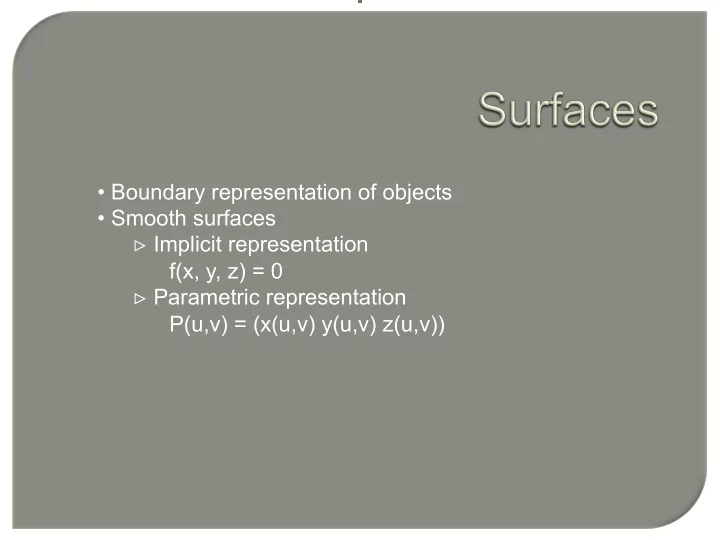
• Boundary representation of objects
• Smooth surfaces

▹ Implicit representation f(x, y, z) = 0 ▹ Parametric representation P(u,v) = (x(u,v) y(u,v) z(u,v))

Parametric Surfaces

P(u,v) = (x(u,v) y(u,v) z(u,v))

• One of the simplest method to generate surfaces
• Obtained by rotating 2D entity about an axis

Point Line parallel to X axis

Circle Cylinder x x y y

Surface of Revolution

Surface of Revolution

Parametric Form

Parametric equation of the entity to be rotated

[ ]

max

t t z(t) y(t) t x t P ≤ ≤ = ) ( ) (

Rotation angle Φ The surface is now a bi-parametric function of two parameters t and Φ Example: Rotation about X – axis of an entity in XY plane Q( t , Φ) = [x(t) y(t)cosΦ y(t)sinΦ]

Surface of Revolution

Sphere is generated by rotating a semi-circle centered at origin and lying in XY plane about X axis Circle: x = rcosθ, y = rsinθ Q (θ,Φ) = [x ycosΦ ysinΦ] = [rcosθ rsinθcosΦ rsinθsinΦ] Similarly ellipsoid is generated by rotating semi ellipse about X axis

Surface of Revolution

Torus is generated by rotating a circle lying in XY plane but whose center does not lie on the axis of rotation. Circle: x = h + rcosθ y = k+ rsinθ Q(θ,Φ)=[h+rcosθ (k+rsinθ)cosΦ (k+rsinθ)sinΦ] (h, k) is the center of the circle

Surface of Revolution

Matrix Form (X axis rotation)

⎥ ⎥ ⎥ ⎥ ⎦ ⎤ ⎢ ⎢ ⎢ ⎢ ⎣ ⎡ = 1 sin cos 1 φ φ S

Φ (x,y) (x, ycosΦ, ysinΦ)

If parametric curve P(t) = FG Then surface of revolution Q(t, Φ)=FGS Can be extended for rotation about any arbitrary axis

Sweep Surfaces

Sweep surfaces are the surfaces generated by traversing an entity along a path in space Q(t,s) = P(t) T(s) T(s) is called the sweep transformation

Sweep Surfaces

Translation sweep of a circle generates a cylinder Translation sweep of a circle accompanied by scaling generates cone

Sweep Surfaces

Example

⎥ ⎥ ⎥ ⎥ ⎦ ⎤ ⎢ ⎢ ⎢ ⎢ ⎣ ⎡ = 1 1 1 1 ) ( ns s T

Translation in Z z x y x y Sweep Surface Cubic Spline

Sweep Surfaces

Normal to the polygon or closed curve as the path is swept can be either kept fixed or it can be made the instantaneous tangent of the curve of sweep.

Fixed normal Tangential normal

Bilinear Interpolation

Linear Interpolation fits the simplest curve between two end points

P1 P2 P(t) = (1-t) P1+ t P2

Bilinear Interpolation

v u b00 b10 b11 b01 u v

Bilinear interpolation fits the simplest surface for the four corner points

Bilinear Interpolation

Two Stage Process

[ ]

⎥ ⎦ ⎤ ⎢ ⎣ ⎡ − ⎥ ⎦ ⎤ ⎢ ⎣ ⎡ − = + − = = + − = + − = v v b b b b u u ub b u v u b v u X vb b v b vb b v b 1 1 ) 1 ( ) , ( ) , ( ) 1 ( ) 1 (

11 10 01 00 01 10 01 00 11 00 11 10 01 10 01 00 01 00

∑ ∑

= =

=

1 1 1 1

) ( ) ( ) , (

i j j i ij

v B u B b v u X

b11 b01 b01 b01

Ruled Surfaces

Given two space curves (C1 & C2) defined in parametric range [0,1], Find a surface X that contains both curves as boundary curves.

) ( ) 1 , ( ) ( ) , (

2 1

u C u X u C u X = =

Many solutions are possible

v u C2 C1

Ruled Surfaces

A simple solution is to do a linear interpolation in v ) 1 , ( ) , ( ) 1 ( ) ( ) ( ) 1 ( ) , (

2 1

u vX u X v u vC u C v v u X + − = + − =

For constant u iso-parametric curve is a line

v u C2 C1

Coon’s Patch

Given Four Boundaries C1(u),C2(u),D1(v),D2(v)

) ( ) , 1 ( ) ( ) , ( ) ( ) 1 , ( ) ( ) , (

2 1 2 1

v D v X v D v X u C u X u C u X = = = = v u C2 C1 D1 D2

Coon’s Patch

C1 C2 rC

Ruled surface between C1(u),C2(u)

Coon’s Patch

C1 C2 rC

Ruled surface between C1(u),C2(u)

D1 D2 rD

Ruled surface between D1(v),D2(v)

Coon’s Patch

C1 C2 rC

Ruled surface between C1(u),C2(u)

D1 D2 rD

Ruled surface between D1(v),D2(v)

+

Coon’s Patch

C1 C2 rC + rD

Ruled surface between C1(u),C2(u)

D1 D2

Ruled surface between D1(v),D2(v)

+

Coon’s Patch

Something is extra which is the bilinear patch formed by the vertices

rCD

Coon’s Patch

C1 D1 D2 C2

+

• Coon’s Patch = rC + rD - rCD

[ ]

⎥ ⎦ ⎤ ⎢ ⎣ ⎡ − ⎥ ⎦ ⎤ ⎢ ⎣ ⎡ − = + − = + − = v v X X X X u u v u r v uX v X u v u r u vX u X v v u r

CD D C

1 ) 1 , 1 ( ) , 1 ( ) 1 , ( ) , ( 1 ) , ( ) , 1 ( ) , ( ) 1 ( ) , ( ) 1 , ( ) , ( ) 1 ( ) , (

Coon’s Patch

Mathematically

Coon’s Patch [ ] [ ] [ ]

⎥ ⎦ ⎤ ⎢ ⎣ ⎡ − ⎥ ⎦ ⎤ ⎢ ⎣ ⎡ − − ⎥ ⎦ ⎤ ⎢ ⎣ ⎡ − + ⎥ ⎦ ⎤ ⎢ ⎣ ⎡ − = v v X X X X u u u X u X v v v X v X u u v u X 1 ) 1 , 1 ( ) , 1 ( ) 1 , ( ) , ( 1 ) 1 , ( ) , ( 1 ) , 1 ( ) , ( 1 ) , (

One can generalize with f1(u)=1-u ,f2(u)=u and g1(v)=1-v,g2(v)=v

Mathematically X(u,v)= rC + rD - rCD

Parametric Surfaces

P(u,v) = (x(u,v) y(u,v) z(u,v))

Bezier Surface

b03 b00 b33 b30

Given control points: b00 b01 …. b33

u v

Bezier Surface

b0 b1 b2 b3 : Control Polygon P(t) b0 b1 b2 b3

1 ) ( ) ( ≤ ≤ = ∑

=

t t J b t P

n i n i i

Mathematically Bezier Curve (Revisit)

The de Casteljau Algorithm

b1 b2 b0 b0

1

b1

1

b0

2

t 1

2 2 1 2 1 1 1 2

) 1 ( 2 ) 1 ( ) ( ) ( ) 1 ( ) ( b t b t t b t t tb t b t t b + − + − = + − =

Bezier Surface

Bezier Curve (Revisit)

2 1 1 1 1 1

) 1 ( ) ( ) 1 ( ) ( tb b t t b tb b t t b + − = + − =

Bezier Surface

Bezier Curve is constructed using successive linear interpolation Bezier Surface can be constructed using successive bi-lineear interpolation

The de Casteljau Algorithm Bezier Curve (Revisit)

Bilinear Interpolation(Revisit)

Two Stage Process

[ ]

⎥ ⎦ ⎤ ⎢ ⎣ ⎡ − ⎥ ⎦ ⎤ ⎢ ⎣ ⎡ − = + − = = + − = + − = v v b b b b u u ub b u v u b v u X vb b v b vb b v b 1 1 ) 1 ( ) , ( ) , ( ) 1 ( ) 1 (

11 10 01 00 01 10 01 00 11 00 11 10 01 10 01 00 01 00

∑ ∑

= =

=

1 1 1 1

) ( ) ( ) , (

i j j i ij

v B u B b v u X

b11 b01 b10 b00

Bezier Surface

u v

b03 b00 b33 b30

u v De Castelejau Algorithm

Bezier Surface

[ ]

⎥ ⎦ ⎤ ⎢ ⎣ ⎡ − ⎥ ⎦ ⎤ ⎢ ⎣ ⎡ − = v v b b b b u u b 1 1

11 10 01 00 11 00

b03 b00 b33 b30

u v De Castelejau Algorithm

Bezier Surface

b03 b00 b33 b30

u v De Castelejau Algorithm

Bezier Surface

[ ]

⎥ ⎦ ⎤ ⎢ ⎣ ⎡ − ⎥ ⎦ ⎤ ⎢ ⎣ ⎡ − = v v b b b b u u b 1 1

11 11 11 10 11 01 11 00 22 00

b03 b00 b33 b30

u v De Castelejau Algorithm

Bezier Surface

b03 b00 b33 b30

u v De Castelejau Algorithm

Bezier Surface

[ ]

⎥ ⎦ ⎤ ⎢ ⎣ ⎡ − ⎥ ⎦ ⎤ ⎢ ⎣ ⎡ − = v v b b b b u u b 1 1

22 11 22 10 22 01 22 00 33 00

33 00

b

Mathematically

[ ]

r) (n 0,1, j i n 2, 1, r v v b b b b u u b

r r j i r r j i r r j i r r j i r r j i

− = = ⎥ ⎦ ⎤ ⎢ ⎣ ⎡ − ⎥ ⎦ ⎤ ⎢ ⎣ ⎡ − =

− − + + − − + − − + − −

• ,

1 1

1 , 1 1 , 1 1 , 1 , 1 1 , 1 1 , 1 , 1 , , ,

De Castelejau Algorithm

Bezier Surface

Problem: If degree in u is not equal to the degree in v

u v

b00 b20 b23 b03

De Castelejau Algorithm

Bezier Surface

A surface can be thought of as being swept out by a moving and deforming curve

Tensor Product

Bezier Surface

∑

=

=

m i m i i m

u B b u b ) ( ) (

∑

=

= =

n j n j j i i i

v B b v b b

,

) ( ) (

Each control point bi traverses a Bezier curve

Tensor Product

Bezier Surface

Let the sweep curve be:

∑ ∑

= =

=

m i n j n j m i j i n m

v B u B b v u b

, ,

) ( ) ( ) , (

Combining Tensor Product

Bezier Surface

Tensor Product

Bezier Surface

Tensor Product

Bezier Surface

Bezier control net

Bezier Surface

Matrix Form

[ ]

⎥ ⎥ ⎥ ⎦ ⎤ ⎢ ⎢ ⎢ ⎣ ⎡ ⎥ ⎥ ⎥ ⎦ ⎤ ⎢ ⎢ ⎢ ⎣ ⎡ = = ∑ ∑

= =

) ( ) ( ) ( ) ( ) ( ) ( ) , (

00 ,

v B v B b b b b u B u B v B u B b v u b

n n n mn m n m m m n j m i m i ij n j n m

Bezier Surface

Properties

• Affine invariance
• Convex hull
• Boundary curve and end-point interpolation
• Change in control point position changes surface

shape

Degree Elevation

Bezier Surface

Degree in u = 2 in v = 3 u v

Degree Elevation

Bezier Surface

Degree in u = 3 in v = 3 u v

Bezier Surface

Bicubic Patch

Bezier Surface

Shape Control

Bezier Surface

Derivatives

ij j i ij n j m i n j m i ij n j n j m i m i ij n m

b b b v B u B b m v B u B b u v u b u − = = ⎥ ⎦ ⎤ ⎢ ⎣ ⎡ ∂ ∂ = ∂ ∂

+ = − = − = =

∑ ∑ ∑ ∑

1 , 1 1 1 , 1 ,

Δ ) ( ) ( Δ ) ( ) ( ) , (

Bezier Surface

Derivatives

ij ij ij m i n j m i n j ij m i m i n j n j ij n m

b b b u B v B b n u B v B b v v u b v − = = ⎥ ⎦ ⎤ ⎢ ⎣ ⎡ ∂ ∂ = ∂ ∂

+ = − = − = =

∑ ∑ ∑ ∑

1 1 , 1 1 1 , ,

Δ ) ( ) ( Δ ) ( ) ( ) , (

Bezier Surface

Derivatives

Cross Boundary Derivatives

b03 b00 b33 b30

30 1 ,

Δ b

) , ( ) , ( ) , ( ) , ( ) , (

, , , ,

v u b v v u b u v u b v v u b u v u n

n m n m n m n m

∂ ∂ × ∂ ∂ ∂ ∂ × ∂ ∂ = u ∂ ∂ v ∂ ∂

Bezier Surface

Normal Vectors

n

Derivatives

∑ ∑

− = − = − −

= ∂ ∂ ∂

1 1 1 1 , 1 , 1 , 2

) ( ) ( Δ ) , (

m i n j n i m j j i n m

v J u J b mn v u b v u

Bezier Surface

Derivatives:

) ( ) ( ) (

, 1 , 1 , 11 , 1 , , 1 1 , 1 , 11 , 1 , , 1 , j i j i j i j i j i j i j i j i j i j i j i j i

P b b b b b b b b b b P − = Δ − − − = Δ − = −

+ + + + + + + +

Geometric Interpretation:

11

Δ

bi,j bi+1,j bi+1,j+1 bi,j+1 Pi,j

Twist Vector

Bezier Surface

Composite Patches

Bezier Surface

Composite Patches C0 Continuous

Bezier Surface

Composite Patches C1 Continuous

Bezier Surface

Utah Teapot 32 Bicubic Bezier patches

B-Spline Surface B-Splines

Polynomial spline function of order k (degree k-1)

1 2 ) ( ) (

max min 1 1 ,

+ ≤ ≤ ≤ ≤ = ∑

+ =

n k t t t t N B t P

n i k i i

Bi : Control point Nik : Basis function

B-Spline Surface

) ( ) ( ) , (

, 1 1 , 1 1

v N u N B v u P

q j m i p i ij n j

∑ ∑

+ = + =

=

Bij : Control point Nip, Njq : Basis functions

B-Spline Surface

Properties

• Affine invariance
• Convex hull (stronger)
• Change in control point position changes surface

shape (local control)

B-Spline Surface

Properties

• local control

B-Spline Surface

Examples

Polygonal Representation

For rendering often object is represented as collection of polygons

Object Surfaces Polygonal Mesh

Polygonal Representation

Polygonal mesh is a collection of edges, vertices and polygons such that each edge is shared by at most two polygons Edge: Connects two vertices Polygon: Closed sequence of edges

Polygonal Representation

Explicit Representation Each polygon is represented by P=((x1,y1,z1) (x2,y2,z2) … (xn,yn,zn)) i.e. vertices are stored in the order of traversal Edges connect the successive vertices plus the last one This representation has restrictive manipulation and has multiple storage of points.

Polygonal Representation

Pointer to Vertex List Each vertex is stored once in a list V V=((x1,y1,z1) (x2,y2,z2) … (xn,yn,zn)) Each polygon is represented as P=(V1,V2,V3) e.g. P1=(1,2,4) and P2=(4,2,3) In this representation it is difficult to find polygons that share an edge.

V4 V2 V3 V1 P1 P2

Polygonal Representation

Pointer to Edge List Edge: E = (Vi,Vj,Pm,Pn) Polygon=(Ep,Eq,Er) V = (V1,V2,V3,V4) E1 = (V1,V2,P1,null) E2 = (V2,V3,P2,null) E3 = (V3,V4,P2,null) E4 = (V4,V2,P1,P2) P1= (E1E4E5) E5 = (V4,V1,P1,null) P2= (E2E3E4)

V4 V2 V3 V1 P1 P2 E4 E1 E5 E3 E2

Polygonal Representation

Winged Edge Data Structure

Edge a Vertices Start X End Y Faces Left 1 Right 2 Left Traverse Pred b Succ d Right Traverse Pred e Succ c