BOD Modeling "L" is modelled as a simple 1st order decay: - - PDF document

CEE 577 Lecture #13 10/23/2017 1

Lecture #13 BOD and Deoxygenation

(Chapra, L20)

Dave Reckhow (UMass) CEE 577 #13 1

Updated: 23 October 2017

Print version

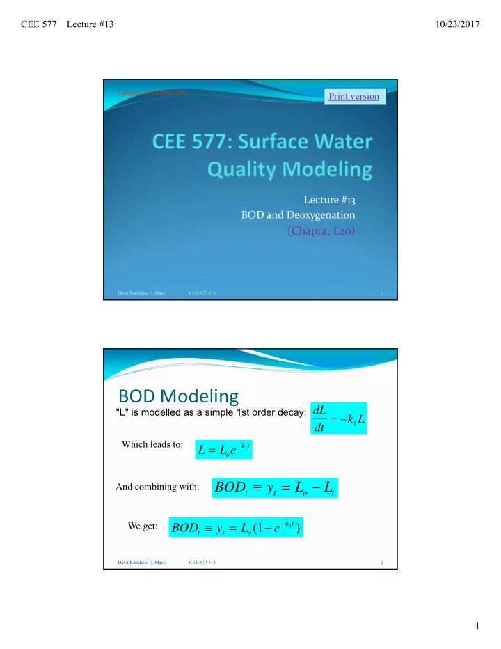
BOD Modeling

Dave Reckhow (UMass) CEE 577 #13 2

"L" is modelled as a simple 1st order decay: dL

dt k L  

1

L L e

• k t



 1

Which leads to: We get:

BOD y L e

t t

• k t

  



( ) 1

1

BOD y L L

t t

• t

  

And combining with:

CEE 577 Lecture #13 10/23/2017 2

Temperature Effects

Dave Reckhow (UMass) CEE 577 #13 3

Temperature Dependence  Chemist's Approach: Arrhenius Equation

d k dT E RT

a a a

(ln ) 

2

k k e

T K E T RT

a

• a

a a



 293 293 293 ( )/

 Engineer's Approach:

k k

T C T C

• 

 20 20



Often we use: =1.047 for CBOD

NBOD

Dave Reckhow (UMass) CEE 577 #13 4

Nitrogeneous BOD (NBOD)

NH O NO H O H

Nitrosomonas 3 2 2 2

15       

 

.

NO O NO

Nitrobacter 2 2 3

1 2

 

    

2 moles oxygen/1 mole of ammonia 4.57 grams oxygen/gram ammonia-nitrogen Like CBOD, the NBOD can be modelled as a simple 1st

• rder decay:

dL dt k L

N N N

 

CEE 577 Lecture #13 10/23/2017 3

NBOD cont.

 The model is then:

 where:

 Nitrifiers

 very slow generation time (~1 day)  sensitive to low D.O.

 NBOD may be very important for non‐nitrified,

but otherwise highly treated waters

Dave Reckhow (UMass) CEE 577 #13 5

 

t k N

• t

N

e L NBOD



  1

 

N NH N

• rg

NBOD L

u N

• 

   

3

57 . 4

Typical Municipal WW Charact.

Dave Reckhow (UMass) CEE 577 #13 6

Parameter Typical Wastewater Characteristics, mg/L except pH U.S. EPA Discharge Standards, mg/L except pH Typical Concentrations in Lakes or Streams, mg/L except pH BOD5 150-300 30 2-10 Total Suspended Solids 150-300 30 2-20 COD 400-600 N/A 5-50 D.O. 4-5 4-Sat. NH3-N 15-40 * <1 NO_ 3 * <1 pH 6-8 6-9 6-8

CEE 577 Lecture #13 10/23/2017 4

BOD Model

Dave Reckhow (UMass) CEE 577 #13 7

    L t U L x k L

r

  

k k k

r d s

 

 v H

s

Decomposition rate in the stream Settling rate   L t  0

L L e

• k xU

r





Estimating the k’s

0.2 0.4 0.6 0.8 1 1.2 1.4 2 4 6 Ln L t* = x/U

Deep Stream Shallow Stream

Dave Reckhow (UMass) CEE 577 #13 8

kd ks+kd k C H H ft k C H ft

d d

          



8 8 8

0 434 .

, ,

  1047 .

Where: C=0.2 for unstable bottoms C=0.3 for rocky bottoms

CEE 577 Lecture #13 10/23/2017 5

Typical DO Sag Curve

Dave Reckhow (UMass) CEE 577 #13 9

2 4 6 8 10 12

• 2

2 4 6 8 D.O. (mg/L) Distance Downstream (miles) Critical Concentration Critical Distance Recovery Zone

Saturation D.O.

Decomposition Dominates Reaeration Dominates

Lecture #22 (Distributed Systems, time variable. Dye Studies)

Chapra, L10

Updated: 23 October 2017

Print version

CEE 577 Lecture #13 10/23/2017 6

Plug Flow (time variable)

 Simulating accidental spill, tracer studies  when a spill causes a concentration of co at x=0

and t=0

David Reckhow CEE 577 #22 11

    c t U c x kc   

c c e

• kt





*

Where: t*=x/U Refer to Example 10.1

David Reckhow CEE 577 #22 12

x1 x2 x3

t=0 t=1 t=2

Moving vs. Fixed frame of reference

CEE 577 Lecture #13 10/23/2017 7

David Reckhow CEE 577 #22 13 u-3s u-2s u-s u u+s u+2s u+3s

Relative Frequency

0.000 0.002 0.004 0.006 0.008 0.010 0.012 0.014 0.016 0.018

68.3% 95.4% 99.7%

The random walk: a normal distribution

Spill Models

 Dispersion and advection

 a normal distribution with:

David Reckhow CEE 577 #22 14

 

c x t m Et e

p x Ut Et

( , ) 

 

2

2

4



m Ac

x Ut Et    2 Equ# 10.24 in Chapra

CEE 577 Lecture #13 10/23/2017 8

Recall from our discussion on Longitudinal Dispersion (~Lecture #9)

 From Fischer et al., 1979

David Reckhow CEE 577 #22 15

E U B HU  0 011

2 2

.

*

Where the Shear Velocity is:

U gHS

* 

m2s-1 m/s Width (m) Mean depth (m)

Empirical Method

 From Dye Study data

 Method of moments

 2 = variance of the concentration‐time curve  t‐bar = time of travel to the centroid of the curve

 The first moment about the origin gives:

 where t0.01 is the time at which concentration has

decreases to 1% of the peak

David Reckhow CEE 577 #22 16

u d tu td x

t t U E   

2 2 2

2  

t U t U t E t E

t t l x x l

     

2 2 2 2 2

2 2 2 2    

Over length, at a single time Over time, at a specific location

 



01 . 01 .

t t

sdt stdt t

CEE 577 Lecture #13 10/23/2017 9

Empirical Method (cont.)

And the 2nd moment about the centroid

gives:

For discrete data these become:

David Reckhow CEE 577 #22 17

2 2 2

) (

01 . 01 .

t sdt dt st

t t

 

 



   

 

 

s st t s t st t

   

2 2 2 2 2

t s st t t s t st    

   

 



Compare to T&M equ 10.32 Compare to T&M equ 10.33

Dye Studies (cont.)

 Single point method

 Use of peak concentration (cp) and time to reach

peak (tp)

 plot cp vs (tp)‐0.5 to get a slope that is a function

• f Ex

 see sample problem 2.6 in T&M (pg. 78)

David Reckhow CEE 577 #22 18

 

5 .

2





p x p

t E A M c 

CEE 577 Lecture #13 10/23/2017 10

Homework #4

 Velocity  dispersion

coefficient

David Reckhow CEE 577 #22 19

USGS Guidelines: Input

 The USGS recommends the following volume or

mass of Rhodamine WT‐20% dye:

David Reckhow CEE 577 #22 20 p m dye

S U x Q x V

93 . 4

10 4 . 3       



dye dye

V W 62 . 2  Liters cfs Miles downstream

Peak concentration desired at distance “x”

ft/sec lb

CEE 577 Lecture #13 10/23/2017 11

USGS Guidelines: Sampling

 Duration of

dye cloud as a function of travel time to peak, and average channel width‐depth ratio (B/H).

David Reckhow CEE 577 #22 21

 To next lecture

Dave Reckhow (UMass) CEE 577 #13 22