
SLIDE 1
BNP survival regression with variable dimension covariate vector
Peter M¨ uller, UT Austin
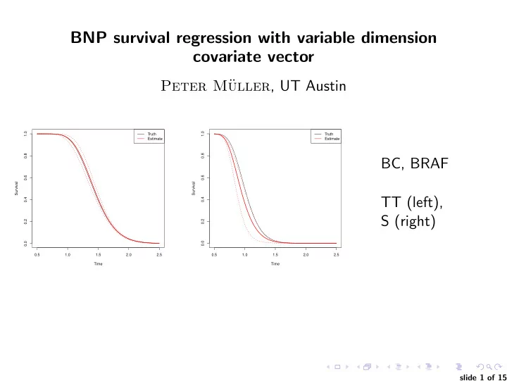
0.5 1.0 1.5 2.0 2.5 0.0 0.2 0.4 0.6 0.8 1.0 Time Survival Truth Estimate 0.5 1.0 1.5 2.0 2.5 0.0 0.2 0.4 0.6 0.8 1.0 Time Survival Truth Estimate
BC, BRAF TT (left), S (right)
slide 1 of 15