Black-Scholes Price The value at time t of a European option whose - - PowerPoint PPT Presentation

Black-Scholes Price

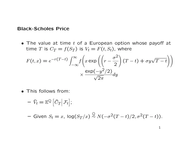
• The value at time t of a European option whose payoff at

time T is CT = f(ST) is Vt = F(t, St), where F(t, x) = e−r(T−t)

∞

−∞f

• x exp
• r − σ2

2

• (T − t) + σy

√ T − t

• × exp(−y2/2)

√ 2π dy

• This follows from:

– ˜ Vt = EQ ˜ CT

• Ft
• ;

– Given St = x, log(ST/x) Q ∼ N(−σ2(T − t)/2, σ2(T − t)).

1

European call

• If f(ST) = (ST − K)+, then

F(t, x) = xΦ(d1) − Ke−r(T−t)Φ(d2), where Φ is the cdf of the standard normal distribution, and (d1, d2) = log

x

K

• +
• r ± σ2

2

• (T − t)

σ√T − t

• Note that the price depends on the volatility σ; could be:

– estimated from historical data: historical volatility; – inferred from other option prices: implied volatility.

2

Replicating the claim CT

• Write ˜

F(t, x) = e−rtF(t, xert); then ˜ Vt = ˜ F(t, ˜ St).

• So

˜ F(t, x) = EQ[ ˜ F(T, ˜ ST)|˜ St = x].

• Because d˜

St = σ ˜ StdXt, the Feynman-Kac representation im- plies that ∂ ˜ F ∂t (t, x) + 1 2σ2x2∂2 ˜ F ∂x2 (t, x) = 0.

3

• By Itˆ
• ’s rule,

˜ F(T, ˜ ST) = ˜ F(0, ˜ S0) +

T

∂ ˜ F ∂x (t, ˜ St)d˜ St +

T

• ∂ ˜

F ∂t (t, ˜ St) + 1 2σ2 ˜ S2

t

∂2 ˜ F ∂x2 (t, ˜ St)

• dt

and the second integral vanishes.

• So

φt = ∂ ˜ F ∂x (t, ˜ St) = ∂F ∂x (t, St).

• In particular, for a European call,

φt = ∂F ∂x (t, x) = Φ(d1).

4

The Greeks

• Let π(t, x) be the value of a portfolio consisting of an asset

with price St = x and derivatives of (contingent claims based

• n) the asset.
• The Greeks are:

Delta: ∆ = ∂π ∂x Gamma: Γ = ∂2π ∂x2 Theta: Θ = ∂π ∂t Vega (really nu):

ν = ∂π

∂σ

5

Foreign Exchange

• How to price contracts and options on a foreign currency.
• Suppose the domestic interest rate is r, the foreign interest

rate is y, and the exchange rate is a geometric Brownian motion: Domestic bond: Bt = ert; Foreign bond: Dt = eut; Exchange rate: Et = E0 exp(νt + σWt), where {Wt}t≥0 is P-Brownian motion.

6

• The exchange rate is not tradable, but St = DtEt, the do-

mestic value on day t of one foreign bond, is tradable. – Conveniently, it is also a GBM, so our existing methods can be used.

• The discounted value process {˜

St}t≥0 satisfies ˜ St = e−rtSt = E0 exp[(−r + u + ν)t + σWt] and is also a GBM.

7

• Define Q by

dQ dP

• Ft

= exp

• θWt − 1

2θ2t

• ,

where θ =

• −r + u + ν + 1

2σ2

• /σ.
• Then by Girsanov’s theorem

Xt

△

= Wt + θt is a Q-Brownian motion, and ˜ St = E0 exp

• σXt − 1

2σ2t

• is a Q-martingale.

8

• Example: a forward contract. We agree to buy one unit of

foreign currency at time T with a strike price K.

• Payoff is CT = ET − K, and the value of this at time t = 0 is

EQ[ ˜ CT] = e−uTE0 − e−rTK.

• Forward contracts are structured so that no money changes

hands up front, so the strike must be K = e(r−u)TE0.

9

• Clearly the hedge is:

– At t = 0 ∗ sell short e−uT foreign bonds; ∗ convert the proceeds to domestic at E0; ∗ buy e−uTE0 = e−rTK domestic bonds. – At t = T ∗ sell the domestic bonds for K; ∗ exchange for one unit of foreign currency under the con- tract; ∗ use it to close the short position in the foreign bond.

10

• From the perspective of a foreign investor, the fair strike K

is the same, and the hedge is the same. – The risk-neutral measure Q is different, but that is a tech- nicality caused by the change of numeraire.

11

Dividends

• The basic Black-Scholes theory is for a stock that pays no

dividends. – Many stocks do not pay dividends, e.g. Microsoft (for some years after IPO), Apple (recently announced re- sumption of its dividend).

• When a stock pays a dividend that is proportional to the

stock price, either continuously or at discrete times, immedi- ate reinvestment creates a portfolio with changing amounts

• f stock.

12

• If the stock price is GBM, so is the portfolio value.
• A fixed dividend is more realistic, but does not yield closed

form solutions.

13

Bonds

• U.S. Treasury bonds have no default risk.

– Their value depends on interest rates: value rises when rates fall.

• Corporate bonds have both interest rate risk and default risk.
• A zero coupon (or discount) bond pays its principal amount

at maturity, and nothing else. – Its value depends only on the rate for deposits to matu- rity T.

14

• Most bonds also make interest (or coupon) payments at in-

termediate times. – The value of a coupon-bearing bond depends on the in- terest rates for deposits to each of its payment dates. – Valuing a bond option requires a model for the whole yield curve (i.e., for the term structure of interest rates).

• For both discount and coupon bonds, GBM is inadequate for

many reasons, including its failure to capture pull to par: – As the bond approaches maturity, its value converges to its face amount, which is certain to be paid.

15

What is tradable?

• A process {Vt}t≥0 is tradable if it is the value of some self-

financing portfolio. – For instance, in the FX example, St = DtEt is tradable, because we can buy one foreign bond at t = 0 and hold it. – But the exchange rate Et is not tradable, because there is no such portfolio.

• Can we make that less heuristic?

16

• Given a riskless cash bond {Bt}t≥0 and a tradable asset

{St}t≥0, a process {Vt}t≥0 represents a tradable asset if and

• nly if the discounted value {B−1

t

Vt}t≥0 is a

• Q, {FS

t }t≥0

• martingale, where Q is the measure under which the dis-

counted asset price {B−1

t

St}t≥0 is a martingale.

• Proof (of “if”):

– by the martingale representation theorem, there exists a predictable {φt}t≥0 such that d˜ Vt = φtd˜ St; – if ψt = ˜ Vt − φt ˜ St, then Vt = φtSt + ψtBt, and the portfolio can be shown to be self-financing. – So {Vt}t≥0 is the value of a self-financing portfolio.

17

• Proof (of “only if”):

– if {Vt}t≥0 is the value of a self-financing portfolio, then there exist predictable {φt}t≥0 and {ψt}t≥0 such that Vt = φtSt + ψtBt; – as shown earlier, the self-financing property dVt = φtdST + ψtdBt implies that d˜ Vt = φtd˜ St, so {˜ Vt}t≥0 is a

• Q, {FS

t }t≥0

• martingale.

18

Market price of risk

• Suppose that multiple risky securities {Si

t}t≥0 trade in a mar-

ket driven by a single P-Brownian motion {Wt}t≥0: dSi

t = µiSi t + σiSi tdWt.

• Then their discounted processes must be Q-martingales for

the same risk neutral measure Q.

• That is,

Xt = Wt +

• µi − r

σi

• t

for each i.

19

• So

γ = µi − r σi is the same for each security; it is a characteristic of the market, not of the individual security.

• The quantity γ is called the market price of risk: the excess

mean return of an asset over the risk free rate per unit risk. – It is essentially the same as the Sharpe ratio.

20