Binary images Constrained image capture setting Two pixel values - - PDF document

binary images
SMART_READER_LITE
LIVE PREVIEW

Binary images Constrained image capture setting Two pixel values - - PDF document

Sudheendras office hours Mon, Wed 1-2 pm Lecture 3: Binary image analysis ENS 31NR Forsyth and Ponce book Thursday, Sept 6 Binary images Constrained image capture setting Two pixel values Foreground and background


slide-1
SLIDE 1

Lecture 3: Binary image analysis

Thursday, Sept 6

  • Sudheendra’s office hours

– Mon, Wed 1-2 pm – ENS 31NR

  • Forsyth and Ponce book

Binary images

  • Two pixel values
  • Foreground and background
  • Regions of interest

Constrained image capture setting

  • R. Nagarajan et al. A real time marking inspection scheme

for semiconductor industries, 2006

Documents, text Medical, bio data

slide-2
SLIDE 2

Intermediate low-level cues

  • =

Edges Motion Orientation

NASA robonaut http://robonaut.jsc.nasa.gov/status/October_prime.htm

Shape

Silhouette visual hulls Medial axis

Outline

  • Thresholding
  • Connected components
  • Morphological operators
  • Region properties

– Spatial moments – Shape

  • Distance transforms

– Chamfer distance

Thresholding

  • Grayscale -> binary mask
  • Useful if object of interest’s intensity

distribution is distinct from background

  • Examplehttp://homepages.inf.ed.ac.uk/rbf/CVonline/LOCAL_COPIES/FITZ

GIBBON/simplebinary.html

Selecting thresholds

  • Partition a bimodal histogram
  • Fit Gaussians
  • Dynamic or local thresholds

A nice case: bimodal intensity histograms

Ideal histogram, light object on dark background Actual observed histogram with noise

Images: http://homepages.inf.ed.ac.uk/rbf/CVonline/LOCAL_COPIES/OWENS/LECT2/node3.html

slide-3
SLIDE 3
  • Example
  • Thresholding a bimodal histogram
  • Otsu method (1979) : automatically select

threshold by minimizing the weighted within-group variance of the two groups of pixels separated by the threshold.

A nice case: bimodal intensity histograms

Not so nice cases

  • Threshold selection is an art, not a science

Shapiro and Stockman

Connected components

  • Identify distinct regions

Shapiro and Stockman

Connected components

  • P. Duygulu

Connectedness

  • Which pixels are considered neighbors

Image from http://www-ee.uta.edu/Online/Devarajan/ee6358/BIP.pdf

4-connected 8-connected

Connected components

  • Various algorithms to compute

– Recursive (in memory) – Two rows at a time (image not necessarily in memory) – Parallel propagation strategy

slide-4
SLIDE 4

Recursive connected components

  • Demo http://www.cosc.canterbury.ac.nz/mukundan/covn/Label.html
  • Find an unlabeled pixel, assign it a new

label

  • Search to find its neighbors, and

recursively repeat to find their neighbors til there are no more

  • Repeat

Sequential connected components

Slide from J. Neira

Morphological operators

  • Dilation
  • Erosion
  • Open, close

Dilation

  • Expands connected components
  • Grow features
  • Fill holes

Before dilation After dilation

Structuring elements

  • Masks of varying shapes used to perform

morphology

  • Scan mask across foreground pixels to

transform the binary image

etc

slide-5
SLIDE 5

Dilation / Erosion

  • Dilation: if current pixel is

foreground, set all pixels under S to foreground in

  • utput (OR)
  • Erosion: if every pixel

under S is foreground, leave as is; otherwise, set current pixel to background in output

Example for Dilation (1D)

SE x f x g ⊕ = ) ( ) (

1 1 1 1 1 1

Input image Structuring Element

1 1

Output Image

1 1 1

Adapted from T. Moeslund

Example for Dilation

1 1 1 1 1 1

Input image Structuring Element

1 1

Output Image

1 1 1

Example for Dilation

1 1 1 1 1 1

Input image Structuring Element

1 1

Output Image

1 1 1

Example for Dilation

1 1 1 1 1 1

Input image Structuring Element

1 1

Output Image

1 1 1

Example for Dilation

1 1 1 1 1 1

Input image Structuring Element

1 1 1 1 1

Output Image

1 1 1

slide-6
SLIDE 6

Example for Dilation

1 1 1 1 1 1

Input image Structuring Element

1 1 1 1 1 1

Output Image

1 1 1

Example for Dilation

1 1 1 1 1 1

Input image Structuring Element

1 1 1 1 1 1 1

Output Image

1 1 1

Example for Dilation

1 1 1 1 1 1

Input image Structuring Element

1 1 1 1 1 1 1

Output Image

1 1 1

Example for Dilation

1 1 1 1 1 1

Input image Structuring Element

1 1 1 1 1 1 1 1 1

Output Image

1 1 1

The object gets bigger and holes are filled!

Erosion

  • Erode connected components
  • Shrink features
  • Remove bridges, branches, noise

Before erosion After erosion

Example for Erosion (1D)

1 1 1 1 1 1

Input image Structuring Element Output Image

1 1 1

SE x f x g O ) ( ) ( =

_

slide-7
SLIDE 7

Example for Erosion (1D)

1 1 1 1 1 1

Input image Structuring Element Output Image

1 1 1

SE x f x g O ) ( ) ( =

_

Example for Erosion

1 1 1 1 1 1

Input image Structuring Element Output Image

1 1 1

Example for Erosion

1 1 1 1 1 1

Input image Structuring Element Output Image

1 1 1

Example for Erosion

1 1 1 1 1 1

Input image Structuring Element Output Image

1 1 1

Example for Erosion

1 1 1 1 1 1

Input image Structuring Element

1

Output Image

1 1 1

Example for Erosion

1 1 1 1 1 1

Input image Structuring Element

1

Output Image

1 1 1

slide-8
SLIDE 8

Example for Erosion

1 1 1 1 1 1

Input image Structuring Element

1

Output Image

1 1 1

Example for Erosion

1 1 1 1 1 1

Input image Structuring Element

1

Output Image

1 1 1

Example for Erosion

1 1 1 1 1 1

Input image Structuring Element

1 1

Output Image

1 1 1

The object gets smaller

Dilation / Erosion

  • Dilation: if current pixel is

foreground, set all pixels under S to foreground in

  • utput (OR)
  • Erosion: if every pixel

under S is foreground, leave as is; otherwise, set current pixel to background in output

Images by P. Duygulu

Opening

  • Erode, then dilate
  • Remove small objects, keep original shape

Before opening After opening

Closing

  • Dilate, then erode
  • Fill holes, but keep original shape

Before closing After closing

slide-9
SLIDE 9

Application: blob tracking

Absolute differences from frame to frame Threshold Erode

Application: blob tracking

  • Background subtraction + blob tracking

Application: segmentation of a liver

Slide credit: Li Shen

Region properties

Some useful features can be extracted once we have connected components, including

  • Area
  • Centroid
  • Extremal points, bounding box
  • Circularity
  • Spatial moments
slide-10
SLIDE 10

Area and centroid

Shapiro & Stockman

Circularity

Shapiro & Stockman [Haralick]

Invariant descriptors

[a1, a2, a3,…] [b1, b2, b3,…] Feature space distance

Often want features independent of position, orientation, scale.

Central moments

S is a subset of pixels (region). Central (j,k)th moment defined as:

  • Invariant to translation of S.

Central moments

  • 2nd central moment: variance
  • 3rd central moment: skewness
  • 4th central moment: kurtosis

Axis of least second moment

  • Invariance to orientation?

Need a common alignment Axis for which the squared distance to 2d object points is minimized.

slide-11
SLIDE 11

Distance transform

  • Image reflecting distance to nearest point

in point set (e.g., foreground pixels).

4-connected adjacency 8-connected adjacency

Distance transform

Edge image Distance transform image

Distance transform (1D)

Adapted from D. Huttenlocher

Distance Transform (2D)

Adapted from D. Huttenlocher

Chamfer distance

  • Average distance to nearest feature

Edge image Distance transform image

  • D. Gavrila, DAGM 1999

Chamfer distance

  • D. Gavrila, DAGM 1999

Edge image Distance transform image More on this and

  • ther distances

later

slide-12
SLIDE 12

Generalized distance transforms

  • Same forward/backward algorithm

applicable with different initialization

  • Initialize with function values F(x,y):

The University of Ontario The University of Ontario

Distance Transform vs. Generalized Distance Transform

Assuming

then is standard Distance Transform (of image features) ⎭ ⎬ ⎫ ⎩ ⎨ ⎧ ∞ = . . ) ( W O feature image is p pixel if p F

) ( p F ) ( p D

∞ + ∞ + ∞ +

Locations of binary image features

p

|| || min )} ( || {|| min ) (

) ( :

q p q F q p p D

q F q q

− = + − =

=

Slide credit Y. Boykov

The University of Ontario The University of Ontario

Distance Transform vs. Generalized Distance Transform

For general

is Generalized Distance Transform of

)} ( || {|| min ) ( q F q p p D

q

+ − =

) ( p F

F(p) may represent non-binary image features (e.g. image intensity gradient)

) ( p F

) ( p F ) ( p D

Slide credit Y. Boykov

Location of q is close to p, and F(q) is small there
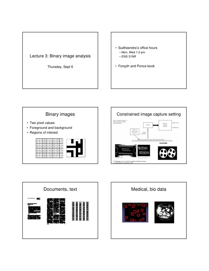
Binary images

  • Pros

– Can be fast to compute, easy to store – Simple processing techniques available – Lead to some useful compact shape descriptors

  • Cons

– Hard to get “clean” silhouettes, noise common in realistic scenarios – Can be too coarse of a representation – Not 3d

Matlab

  • N = HIST(Y,M)
  • L = BWLABEL(BW,N);
  • STATS = REGIONPROPS(L,PROPERTIES) ;

– 'Area' – 'Centroid' – 'BoundingBox' – 'Orientation‘, …

  • IM2 = imerode(IM,SE);
  • IM2 = imdilate(IM,SE);
  • IM2 = imclose(IM, SE);
  • IM2 = imopen(IM, SE);
  • [D,L] = bwdist(BW,METHOD);
  • Everything is matrix

Tutorial adapted from W. Freeman, MIT 6.896

slide-13
SLIDE 13
  • Matrix index
  • Manipulate matrices
  • Manipulate matrices
  • Scripts and functions

– Scripts are m-files containing MATLAB statements – Functions are like any other m-file, but they accept arguments – Name the function file the same as the function name

  • Try to code in matrix ways
  • whos
  • help
  • lookfor
  • clear / clear x
  • save
  • load