Big Transfer (BiT): General Visual Representation Learning Abhash - - PDF document

Big Transfer (BiT): General Visual Representation Learning

Abhash Kumar Singh Harit Vishwakarma

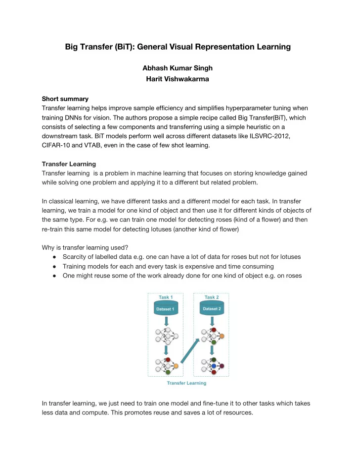
Short summary Transfer learning helps improve sample efficiency and simplifies hyperparameter tuning when training DNNs for vision. The authors propose a simple recipe called Big Transfer(BiT), which consists of selecting a few components and transferring using a simple heuristic on a downstream task. BiT models perform well across different datasets like ILSVRC-2012, CIFAR-10 and VTAB, even in the case of few shot learning. Transfer Learning Transfer learning is a problem in machine learning that focuses on storing knowledge gained while solving one problem and applying it to a different but related problem. In classical learning, we have different tasks and a different model for each task. In transfer learning, we train a model for one kind of object and then use it for different kinds of objects of the same type. For e.g. we can train one model for detecting roses (kind of a flower) and then re-train this same model for detecting lotuses (another kind of flower) Why is transfer learning used?

• Scarcity of labelled data e.g. one can have a lot of data for roses but not for lotuses
• Training models for each and every task is expensive and time consuming
• One might reuse some of the work already done for one kind of object e.g. on roses

In transfer learning, we just need to train one model and fine-tune it to other tasks which takes less data and compute. This promotes reuse and saves a lot of resources.

In transfer learning,

• There is better initial performance on target tasks than random initialization.
• There is higher slope, which means learning is faster on a target task.
• There is higher asymptote, that is the converged model is better than otherwise would

have been. Popularity of Transfer Learning Recently there has been a trend in Transfer Learning where it has become very popular on a task called Named Entity Recognition where models like BERT have achieved state of the art in NLP tasks. Similar trend is observed in the field of Computer Vision. Paper Summary In this paper, vision related tasks have been discussed. On a high level, a model is trained on a generic large supervised dataset and then fine tuned on a target task.

• Scale up pre-training - The authors show how pre-training is achieved on a very large

dataset with large models.

• Fine - tune model to downstream tasks - Then this model is fine tuned to downstream

tasks by using less data and compute. Only a few hyperparameters are used in this approach called BiT-HyperRule. BiG Transfer (BiT) There are two components - upstream training, where the model is pre-trained, and downstream training where the previous trained model is fine- tuned. Upstream components

• Large scale dataset and model - There are 3 different datasets mentioned below, which

are used for pre-training. Their related information is mentioned below.

• Normalization - We usually normalize activations along a subset of (N,C,H,W)
• dimensions. [ N - data points in a batch, C - channels, H - height of image, W - width of

image]. It has been shown that this leads to faster and stable training of DNN by making loss function smooth.

In Batch Norm, we normalize over data points and not over channels, so you’re doing it independently for each channel. In Layer Norm, you’re normalizing over channels for each data point. In Instance Norm, you’re normalizing for one channel and one data point. In Group Norm, you’re normalizing over groups of channels for each data point. LN and IN are special cases of GN. GN is more effective than BN when batch size is small. Reason is in BN, we are normalizing over data points and since batch size is small, we can’t get a good approximation of mean and variance.

• Weight Standardization - This is a recent technique developed, where weights are

normalized instead of activations. It helps in smoothing the loss landscape and works well in conjunction with GN in a low batch size regime. Upstream training is summarized below :

Downstream Components In this part, we transfer the learned model to different tasks and the goal here is cheap fine-tuning. We should not be using a lot of data and compute resources. Also, there should not be a lot of hyperparameter tuning involved. BiT- HyperRule

• Most hyperparameters need not be changed
• Depending on dataset size and image resolution, set training schedule length, image

resolution and MixUp regularization.

• The tasks are divided into small, medium and large depending on the number of training

instances. The downstream fine-tuning is summarized below : MixUp Regularization MixUp regularization is a way to introduce new samples which are convex combination of existing samples.

Here we see that there are two classes - green is negative class and yellow is positive class. If we train ERM, we can see that the blue region [indicates P(y=1|x) ] is tightly concentrated along the labels but when MixUp regularization is used, we see a smoothed gradient towards the

• ther class.

This technique is shown to improve generalization and reduce memorization of corrupt labels. It also increases robustness to adversarial examples. In BiT, mixup is used with α = 0.1 for large and medium tasks. Downstream Tasks The authors tested BiT on 5 different downstream tasks summarized below : Results

BiT-L is evaluated on standard benchmarks and top-1 accuracy is reported here. It outperforms previous SOTA along with some SOTA specialist models. Specialist models are those that condition pre-training

• n each task, while generalist models, including BiT, perform task-independent pre-training. Specialist

representations are highly effective, but require a large training cost per task while generalized representations require large-scale training only once, followed by a cheap adaptation phase. ImageNet-21k is more than 10 times bigger than ILSVRC-2012, but it is mostly overlooked by the research community. When BiT-M is trained on it, there is notable performance gain compared to BiT-S which is trained on ILSVRC-2012. The authors performed few shot learning for transferring BiT-L successfully. They evaluated subsets of ILSVRC-2012, CIFAR-10, and CIFAR-100, down to 1 example per class. Even with few samples per class, BiT-L shows strong performance and quickly saturates to performance of full data regime. Graph : The solid line shows the median across results on 5 subsamples per dataset, where every trial is plotted on the graph. We can see that variance is low, except 1-shot CIFAR-10, because it has just 10 images.

The authors tried to compare BiT with semi-supervised learning, although they noted that both approaches are different. Semi-supervised methods have access to extra unlabelled data from the training distribution, while BiT makes use of out-of-distribution labeled data. VTAB [Visual Task Adaptation Benchmark] has 19 tasks with 1000 examples/task. BiT outperforms current SOTA by large margin. The graph compares methods that manipulate 4 hyperparameters vs single BiT-HyperRule. The authors tested BiT models on the ObjectNet dataset. This dataset closely resembles real-life scenarios, where object categories may appear in non-canonical context, viewpoint, rotation etc. They noted that both large architecture and pre-training on more data is crucial to get top-5 accuracy of 80%, almost 25% improvement over previous SOTA. Finally, they evaluated BiT for object detection on the COCO-2017 dataset. They used RetinaNet using pre-trained BiT models as backbones. Instead of using BiT-HyperRule, they stuck with standard RetinaNet training protocol.Here as well, BiT models outperform standard ImageNet pre-trained models.

Usually the norm is that larger neural networks result in better performance. The authors investigated the relation between model size and upstream dataset size on downstream performance. They observed that the benefits of larger models are more on larger datasets(JFM and ImageNet-21k). Also, as evident from the graph, there is a limited benefit of training a large model on a small dataset and training a small model on a large dataset. ResNet50x1 trained on JFT-300M performs worse than when trained on ImageNet21k on CIFAR100 and ISLVRC-2012. In the low data regime, the authors pre-trained on 3 datasets and evaluated on 2 downstream datasets. The line shows the median of 5 runs on random data subsets. BiT-L gives strong results on tiny datasets and on ILSVRC-2012, they outperform models trained on the entire ILSVRC-2012 dataset itself, for the case of 1 example/class.

The authors propose some guidelines on training from large datasets like JFT-300M. First, for getting good performance with large architectures on large datasets, the computational budget should be high. [Left graph] When the budget used for ISLVRC-2012 is applied to ImageNet-21k, the resulting model is

• worse. However, when trained longer, we see improvement.

[Middle graph] On JFT-300M, if we look at 8GPU weeks window, there is not much improvement however if the model is let to train for a longer time window, the improvement is visible. [Dotted graph] When learning rate is decayed too early, final performance is worse. Second, weight decay is an important part of pre-training with large datasets. [Orange Line] Lower weight decay can result in apparent acceleration of convergence. But this leads to an under-performing final model. Low weight decay results in growing weight norms, which in turn results in a diminishing effective learning rate. Current popular methods use BN for training on large datasets with large batch sizes. For BiT, the memory requirement per accelerator is high which translates to small per-device batch sizes. BN performs worse with small batch sizes. Accumulating BN statistics across devices has latency cost and is shown to harm generalization. [Table 4] The authors used GN and WS instead of BN. They found that using only GN leads to performance drop on ILSVRC-2012, but when used with WS, it gave better results. [Table 5] Even on downstream tasks, GN+WS performed better than BN.

Criticism/Future Work Discussion Question from Prof. Sharon Li : Does JFT-300M have class sample disparity (some classes have low number of instances while some have a lot)? Answer - The data distribution of JFT-300M is heavily long-tailed: e.g., there are more than 2M ‘flowers’, 3250 ‘subarau360’ but only 131 images of ‘train conductors’. In fact, the tail is so heavy that it has more than 3K categories with less than 100 images each and approximately 2K categories with less than 20 images per category. Question from ​Rui Huang​ : How do authors handle multiple labels? Answer - When training with multiple labels, we can assign the ground truth label by equally dividing it and assigning same probability to each class and then train using cross - entropy

• loss. ​For evaluation, the authors present top-k accuracy to handle multiple labels.

Question from Prof. Sharon Li​ - Why is learning rate warm up done in upstream training? Answer - The intuition is that in the early stages of learning, we don’t want our model to learn quickly and overfit to examples seen earlier in the training. To deal with this, the learning rate is usually increased incrementally in steps to a final learning rate.