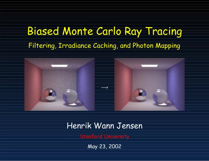
SLIDE 1 Biased Monte Carlo Ray Tracing
Filtering, Irradiance Caching, and Photon Mapping
→ Henrik Wann Jensen
Stanford University May 23, 2002
SLIDE 2 Unbiased and Consistent
Unbiased estimator: E{X} =
Consistent estimator: lim
N→∞ E{X} →
SLIDE 3 Unbiased and Consistent
Unbiased estimator: 1 N
N
f(ξi) Consistent estimator: 1 N + 1
N
f(ξi)
SLIDE 4 Unbiased Methods
- Variance (noise) is the only error
- This error can be analyzed using the variance (i.e.
95% of samples are within 2% of the correct result)
SLIDE 5 Path Tracing (Unbiased)
10 paths/pixel
SLIDE 6 Path Tracing (Unbiased)
10 paths/pixel
SLIDE 7 Path Tracing (Unbiased)
100 paths/pixel
SLIDE 8
How Can We Remove This Noise
SLIDE 9 The World is Diffuse!
Arnold Rendering
SLIDE 10 The World is Diffuse!
Arnold Rendering
SLIDE 11 The World is Diffuse!
Arnold Rendering
SLIDE 12 Noise Reduction/Removal
- More samples (slow convergence, σ ∝ 1/
√ N)
SLIDE 13 Noise Reduction/Removal
- More samples (slow convergence, σ ∝ 1/
√ N)
- Better sampling (stratified, importance, qmc etc.)
SLIDE 14 Noise Reduction/Removal
- More samples (slow convergence, σ ∝ 1/
√ N)
- Better sampling (stratified, importance, qmc etc.)
- Adaptive sampling
SLIDE 15 Noise Reduction/Removal
- More samples (slow convergence, σ ∝ 1/
√ N)
- Better sampling (stratified, importance, qmc etc.)
- Adaptive sampling
- Filtering
SLIDE 16 Noise Reduction/Removal
- More samples (slow convergence, σ ∝ 1/
√ N)
- Better sampling (stratified, importance, qmc etc.)
- Adaptive sampling
- Filtering
- Caching and interpolation
SLIDE 17 Stratified Sampling
Latin Hypercube: 10 paths/pixel
SLIDE 18 Quasi Monte-Carlo
Halton-Sequence: 10 paths/pixel
SLIDE 19 Fixed (Random) Sequence
10 paths/pixel
SLIDE 21 Filtering: Idea
- Noise is high frequency
- Remove high frequency content
SLIDE 22 Unfiltered Image
10 paths/pixel
SLIDE 23 3x3 Lowpass Filter
10 paths/pixel
SLIDE 24 Unfiltered Image
10 paths/pixel
SLIDE 25 3x3 Median Filter
10 paths/pixel
SLIDE 26
Energy Preserving Filters
SLIDE 27 Energy Preserving Filters
- Distribute noisy energy over several pixels
SLIDE 28 Energy Preserving Filters
- Distribute noisy energy over several pixels
- Adaptive filter width
[Rushmeier and Ward 94]
[McCool99]
[Suykens and Willems 00]
SLIDE 29 Problems With Filtering
- Everything is filtered (blurred)
⋆ Textures ⋆ Highlights ⋆ Caustics ⋆ . . .
SLIDE 30
Caching Techniques
SLIDE 31
Caching Techniques
Irradiance caching : Compute irradiance at selected points and inter- polate. Photon mapping : Trace ‘‘photons’’ from the lights and store them in a photon map, that can be used during rendering.
SLIDE 32
Box: Direct Illlumination
SLIDE 33
Box: Global Illlumination
SLIDE 34
Box: Indirect Irradiance
SLIDE 35 Irradiance Caching: Idea
‘‘A Ray Tracing Solution for Diffuse Interreflection’’. Greg Ward, Francis Rubinstein and Robert Clear:
Idea: Irradiance changes slowly → interpolate.
SLIDE 36 Irradiance Sampling
E(x) =
L′(x, ω′) cos θ dω′
SLIDE 37 Irradiance Sampling
E(x) =
L′(x, ω′) cos θ dω′ = 2π π/2 L′(x, θ, φ) cos θ sin θ dθ dφ
SLIDE 38 Irradiance Sampling
E(x) =
L′(x, ω′) cos θ dω′ = 2π π/2 L′(x, θ, φ) cos θ sin θ dθ dφ ≈ π TP
T
P
L′(θt, φp) θt = sin−1
T
P
SLIDE 39 Irradiance Change
ǫ(x) ≤
∂x (x − x0) + ∂E ∂θ (θ − θ0)
SLIDE 40 Irradiance Change
ǫ(x) ≤
∂x (x − x0) + ∂E ∂θ (θ − θ0)
≤ E0 4 π ||x − x0|| xavg +
N(x) · N(x0)
SLIDE 41 Irradiance Interpolation
w(x) = 1 ǫ(x) ≈ 1
||x−x0|| xavg +
N(x) · N(x0) Ei(x) =
wi(x)E(xi)
wi(x)
SLIDE 42
Irradiance Caching Algorithm
Find all irradiance samples with w(x) > q if (samples found) interpolate else compute new irradiance sample
SLIDE 43 Box: Irradiance Caching
1000 sample rays, w>10
SLIDE 44 Box: Irradiance Cache Positions
1000 sample rays, w>10
SLIDE 45 Box: Irradiance Caching
1000 sample rays, w>20
SLIDE 46 Box: Irradiance Cache Positions
1000 sample rays, w>20
SLIDE 47 Box: Irradiance Caching
5000 sample rays, w>10
SLIDE 48 Box: Irradiance Cache Positions
5000 sample rays, w>10
SLIDE 49 Caustics
Pathtracing – 1000 paths/pixel
SLIDE 50
A simple test scene
SLIDE 51
Rendering
SLIDE 52
Photon Tracing
SLIDE 53
Photons
SLIDE 54 Radiance Estimate
L(x, ω) =
fr(x, ω′, ω)L′(x, ω′) cos θ′ dω
SLIDE 55 Radiance Estimate
L(x, ω) =
fr(x, ω′, ω)L′(x, ω′) cos θ′ dω =
fr(x, ω′, ω) dΦ2(x, ω′) dω cos θ′dA cos θ′dω
SLIDE 56 Radiance Estimate
L(x, ω) =
fr(x, ω′, ω)L′(x, ω′) cos θ′ dω =
fr(x, ω′, ω) dΦ2(x, ω′) dω cos θ′dA cos θ′dω =
fr(x, ω′, ω)dΦ2(x, ω′) dA
SLIDE 57 Radiance Estimate
L(x, ω) =
fr(x, ω′, ω)L′(x, ω′) cos θ′ dω =
fr(x, ω′, ω) dΦ2(x, ω′) dω cos θ′dA cos θ′dω =
fr(x, ω′, ω)dΦ2(x, ω′) dA ≈
n
fr(x, ω′
p,
ω)∆Φp(x, ω′
p)
πr2
SLIDE 58 Radiance Estimate
L
SLIDE 59
The photon map datastructure
The photons are stored in a left balanced kd-tree struct photon = { float position[3]; rgbe power; // power packed as 4 bytes char phi, theta; // incoming direction short flags; }
SLIDE 60
Rendering: Caustics
SLIDE 61 Caustic from a Glass Sphere
Photon Mapping: 10000 photons / 50 photons in radiance estimate
SLIDE 62 Caustic from a Glass Sphere
Path Tracing: 1000 paths/pixel
SLIDE 63
Sphereflake Caustic
SLIDE 64 Reflection Inside A Metal Ring
50000 photons / 50 photons in radiance estimate
SLIDE 65 Caustics On Glossy Surfaces
340000 photons / ≈ 100 photons in radiance estimate
SLIDE 66 HDR environment illumination
Using lightprobe from www.debevec.org
SLIDE 67
Cognac Glass
SLIDE 68
Cube Caustic
SLIDE 69 Global Illumination
100000 photons / 50 photons in radiance estimate
SLIDE 70 Global Illumination
500000 photons / 500 photons in radiance estimate
SLIDE 71 Fast estimate
200 photons / 50 photons in radiance estimate
SLIDE 72 Indirect illumination
10000 photons / 500 photons in radiance estimate
SLIDE 73
Global Illumination
SLIDE 74 Global Illumination
global photon map caustics photon map
SLIDE 75 Photon tracing
- Photon emission
- Photon scattering
- Photon storing
SLIDE 76 Photon emission
Given Φ Watt lightbulb. Emit N photons. Each photon has the power Φ
N Watt.
- Photon power depends on the number of emitted
photons. Not on the number of photons in the photon map.
SLIDE 77 What is a photon?
- Flux (power) - not radiance!
- Collection of physical photons
⋆ A fraction of the light source power ⋆ Several wavelengths combined into one entity
SLIDE 78
Diffuse point light
Generate random direction Emit photon in that direction // Find random direction do { x = 2.0*random()-1.0; y = 2.0*random()-1.0; z = 2.0*random()-1.0; } while ( (x*x + y*y + z*z) > 1.0 );
SLIDE 79 Example: Diffuse square light
- Generate random position p on square
- Generate diffuse direction d
- Emit photon from p in direction d
// Generate diffuse direction u = random(); v = 2*π*random(); d = vector( cos(v)√u, sin(v)√u, √1 − u );
SLIDE 80 Surface interactions
The photon is
- Stored (at diffuse surfaces) and
- Absorbed (A) or
- Reflected (R) or
- Transmitted (T)
A + R + T = 1.0
SLIDE 81
Photon scattering
The simple way: Given incoming photon with power Φp Reflect photon with the power R ∗ Φp Transmit photon with the power T ∗ Φp
SLIDE 82 Photon scattering
The simple way: Given incoming photon with power Φp Reflect photon with the power R ∗ Φp Transmit photon with the power T ∗ Φp
- Risk: Too many low-powered photons - wasteful!
- When do we stop (systematic bias)?
- Photons with similar power is a good thing.
SLIDE 83 Russian Roulette
- Statistical technique
- Known from Monte Carlo particle physics
- Introduced to graphics by Arvo and Kirk in 1990
SLIDE 84
Russian Roulette
Probability of termination: p
SLIDE 85
Russian Roulette
Probability of termination: p E{X}
SLIDE 86
Russian Roulette
Probability of termination: p E{X} = p · 0
SLIDE 87
Russian Roulette
Probability of termination: p E{X} = p · 0 + (1 − p)
SLIDE 88
Russian Roulette
Probability of termination: p E{X} = p · 0 + (1 − p) · E{X} 1 − p
SLIDE 89
Russian Roulette
Probability of termination: p E{X} = p · 0 + (1 − p) · E{X} 1 − p = E{X}
SLIDE 90
Russian Roulette
Probability of termination: p E{X} = p · 0 + (1 − p) · E{X} 1 − p = E{X} Terminate un-important photons and still get the correct result.
SLIDE 91
Russian Roulette Example
Surface reflectance: R = 0.5 Incoming photon: Φp = 2 W r = random(); if ( r < 0.5 ) reflect photon with power 2 W else photon is absorbed
SLIDE 92
Russian Roulette Intuition
Surface reflectance: R = 0.5 200 incoming photons with power: Φp = 2 Watt Reflect 100 photons with power 2 Watt instead of 200 photons with power 1 Watt.
SLIDE 93 Russian Roulette
- Very important!
- Use to eliminate un-important photons
- Gives photons with similar power :)
SLIDE 94
Sampling a BRDF
fr(x, ωi, ωo) = w1fr,1(x, ωi, ωo) + w2fr,2(x, ωi, ωo)
SLIDE 95
Sampling a BRDF
fr(x, ωi, ωo) = w1 · fr,d + w2 · fr,s r = random()·(w1 + w2); if ( r < w1 ) reflect diffuse photon else reflect specular
SLIDE 96
Rendering
SLIDE 97
Direct Illumination
SLIDE 98
Specular Reflection
SLIDE 99
Caustics
SLIDE 100
Indirect Illumination
SLIDE 101 Rendering Equation Solution
Lr(x, ω) =
fr(x, ω′, ω)Li(x, ω′) cos θi dω′
i
=
fr(x, ω′, ω)Li,l(x, ω′) cos θi dω′
i +
fr,s(x, ω′, ω)(Li,c(x, ω′) + Li,d(x, ω′)) cos θi dω′
i +
fr,d(x, ω′, ω)Li,c(x, ω′) cos θi dω′
i +
fr,d(x, ω′, ω)Li,d(x, ω′) cos θi dω′
i .
SLIDE 102 Features
- Photon tracing is unbiased
⋆ Radiance estimate is biased but consistent ⋆ The reconstruction error is local
- Illumination representation is decoupled from the
geometry
SLIDE 103 Box
200000 global photons, 50000 caustic photons
SLIDE 104 Box: Global Photons
200000 global photons
SLIDE 105 Fractal Box
200000 global photons, 50000 caustic photons
SLIDE 106
Cornell Box
SLIDE 107
Indirect Illumination
SLIDE 108
Little Matterhorn
SLIDE 109
Mies house (swimmingpool)
SLIDE 110
Mies house (3pm)
SLIDE 111
Mies house (6pm)
SLIDE 112 More Information
Realistic Image Synthesis Using Photon Mapping Realistic Image Synthesis Using Photon Mapping
Realistic Image Synthesis Using Photon Mapping
Realistic Image Synthesis Using Photon Mapping
Foreword by Pat Hanrahan
Realistic Image Synthesis Using Photon Mapping
Henrik Wann Jensen Jensen
Foreword by Pat Hanrahan
The creation of realistic three-dimensional images is central to
computer graphics. Photon mapping, an extension of ray tracing, makes it possible to efficiently simulate global illumination in complex scenes. Photo mapping can simulate caustics (focused light, such as shimmering waves at the bottom of a swimming pool), diffuse inter-reflections (e.g., the `bleeding' of colored light from a red wall onto a white floor, giving the floor a reddish tint), and participating media (e.g., clouds or smoke). This book is a practical guide to photon mapping; it provides both the theory and the practical insight necessary to implement photon mapping and simulate all types of direct and indirect illumination efficiently. A K PETERS LTD.
A K PETERS
Henrik Wann Jensen
http://graphics.stanford.edu/˜henrik henrik@graphics.stanford.edu