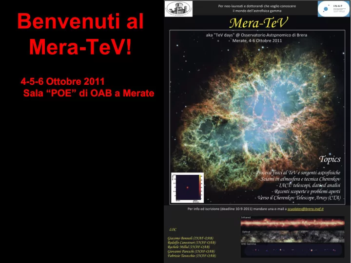
Benvenuti al Mera-TeV! 4-5- -6 Ottobre 2011 6 Ottobre 2011 Sala - - PowerPoint PPT Presentation

Benvenuti al Mera-TeV!

4-5-

• 6 Ottobre 2011

6 Ottobre 2011 Sala “POE” di OAB a Merate Sala “POE” di OAB a Merate

Lorenzo Sironi Lorenzo Sironi

FATE DOMANDE! FATE DOMANDE!

• Le domande sono gradite, anche

prima della fine dei contributi.

• L'incontro è volutamente informale,

e lo spirito è orientato alla comprensione delle tematiche ed alla interazione tra i partecipanti.

SOCIAL EVENT SOCIAL EVENT

w w

Visita alle Cupole Zeiss e Ruths: Visita alle Cupole Zeiss e Ruths: Mercoledì 5, ore 18.15 Mercoledì 5, ore 18.15

SOCIAL DINNER SOCIAL DINNER

• Taverna dei Cacciatori – Imbersago
• Ore 20.00 Mercoledì
• Partenza da Osservatorio ore 19.45

Pranzi e Pause Caffè Pranzi e Pause Caffè

 Pranzi: alle 13.00 nel parco, di fronte

alla Cupola Ruths

 Coffe Breaks: nella Biblioteca, piano

seminterrato edificio principale.

Buon Buon Mera Mera-

• TeV

TeV!! !!

Beaming Beaming

Radio Radio-

• loud AGNs

loud AGNs Gamma Ray Bursts Gamma Ray Bursts ~ 0.1 M ~ 0.1 Mo yr yr-1 G~20 ~20 ~ 10 ~ 10-5 M Mo in a few sec in a few sec G~300 ~300

Lorentz transformations: v along x Lorentz transformations: v along x

x’ = x’ = G (x (x – vt) vt) y’ = y y’ = y z’ = z z’ = z t’ = t’ = G (t (t – v x/c v x/c2)

for for Dt = 0 t = 0  Dx = x = Dx’/ x’/G Contraction Contraction for for Dx’ = 0 x’ = 0  Dt = t = G D G Dt’ t’ time dilation time dilation

Text book special relativity Text book special relativity

x = x = G (x’ + vt’) (x’ + vt’) y = y’ y = y’ z = z’ z = z’ t = t = G (t’ + v x’/c (t’ + v x’/c2)

To remember: mesons created at a height of ~15 km can reach the earth, even if their lifetime is a few microsec  ct’life=hundreds of meters.

v=0 v=0 G=1 =1 v=0.866c v=0.866c G=2 =2

v Can we see contracted spheres? Can we see contracted spheres? Einstein: Yes! Einstein: Yes!

James Terrel 1959 James Terrel 1959 Roger Penrose 1959 Roger Penrose 1959

v=0 v=0 G=1 =1

v

NO! NO!

v=0.866c =0.866c G=2 =2

Relativity with Relativity with photons photons

From rulers and clocks From rulers and clocks to photographs and frequencies to photographs and frequencies

Or: Or: from elementary particles to extended objects from elementary particles to extended objects

The moving square The moving square

b=0 =0 b=0.5 =0.5

Your camera, Your camera, very far away very far away

The moving square The moving square

t=l’/c t=l’/c

vt= vt=bl’ l’ l’/ l’/G

ltot

tot = l’ (

= l’ (b+1/ +1/G) max:2 max:21/2

1/2l’ (diag)

l’ (diag) min: l’ (for min: l’ (for b=0) =0)

l’ l’

l’cos l’cosa = = bl’ l’  cos cosa a = b cos cos(p (p-p/2 p/2-a) = a) = sin sina = 1/G a = 1/G

p/2 p/2-a

a

) ) p/2 p/2-a

p/2 p/2-a

Time Time

CD = c CD = cDte – c cDt tebcos cosq  DtA= = Dte

e (1

(1-bcos cosq) )  DtA= = Dte’ ’ G(1 (1-bcos cosq) ) Dte

e = emission time in lab frame

= emission time in lab frame Dte’ = emission time in comov. frame ’ = emission time in comov. frame Dte

e =

= Dte’ ’ G

Relativistic Doppler factor Relativistic Doppler factor d

DtA= = Dte’ ’ G(1 (1-bcos cosq) ) n= = n’ / ’ / G(1 (1-bcos cosq) )

d

d = 1

G(1

(1-bcos cosq)

Standard Standard relativity relativity Doppler effect Doppler effect

You change frame You remain in lab frame

Relativistic Doppler factor Relativistic Doppler factor d

d =

1

G(1

(1-bcos cosq)

2G for for q=0 =0o

G G for

for q=1/ =1/G G 1/G 1/G for for q=90 90o

=

{

At small angles, Doppler wins over Spec. Relat. At small angles, Doppler wins over Spec. Relat.

Nucleo

bapp

app =

= b b sin sinq 1-

• bcos

cosq = vapp

app =

= v Dte sin sinq

Dte (1

(1-bcos cosq)

Dsapp

app

DtA

q=0 =0o  bapp

app=0

=0

cos cosq=b; ; sin sinq=1/ =1/G  bapp

app=bG

bG

q=90 =90o  bapp

app=b

There is no There is no G.

• G. Correct?

Correct?

Aberration of light Aberration of light

Aberration of light Aberration of light

sin sinq = sin = sinq’/ ’/d dW W = dW’/ ’/d2

sin sinq = sin = sinq’/ ’/d

Aberration of light Aberration of light

K’ K’

dW W = d = dW’/ ’/d2

K

v

Observed vs intrinsic Intensity Observed vs intrinsic Intensity

d3I’( I’(n’) ’)

I( I(n) n3 I’( I’(n’) ’) n’3 = =

invariant invariant

I( I(n) =

I( I(n)

cm cm2

2 s Hz sterad

s Hz sterad

=

erg erg

=

dA dA dt d dt dn dW E

Observed vs intrinsic Intensity Observed vs intrinsic Intensity

d3I’( I’(n’) ’)

I( I(n) n3 I’( I’(n’) ’) n’3 = =

invariant invariant

I( I(n) =

I( I(n)

cm cm2

2 s Hz sterad

s Hz sterad

=

erg erg

=

dA dA dt d dt dn dW E

Observed vs intrinsic Intensity Observed vs intrinsic Intensity

d3I’( I’(n’) ’)

I( I(n) n3 I’( I’(n’) ’) n’3 = =

invariant invariant

I( I(n) =

I( I(n)

cm cm2

2 s Hz sterad

s Hz sterad

=

erg erg

=

dA’ dA’ dW’/d2 E’ E’d

d3I’( I’(n’) ’)

=

I d4I’ I’ = F d4F’ F’ =

d blueshift blueshift d time time d2 aberration aberration

v=0

L=100 W

v=0.995c G=10

L=16MW L=10mW L=0.6mW

v=0.995c G=10

blazars radiogalaxies …….?

v=0.995c G=10

blazars radiogalaxies blazars!

jet counterjet (invisible)

v v

Radiation processes Radiation processes

Radiation processes Radiation processes

• Line emission and radiative transitions in atoms and

Line emission and radiative transitions in atoms and molecules molecules

• Breemstrahlung/Blackbody

Breemstrahlung/Blackbody

• Curvature radiation

Curvature radiation

• Cherenkov

Cherenkov

• Annihilation

Annihilation

• Unruh radiation

Unruh radiation

• Hawking radiation

Hawking radiation

• Synchrotron

Synchrotron

• Inverse Compton

Inverse Compton

V=0 V=0

E

V

( (g=2)

Charge at time Charge at time 9.00 9.00 Contracted sphere… Contracted sphere… E-field lines at time field lines at time 9.00 point to… where 9.00 point to… where the charge is at 9.00 the charge is at 9.00

E

dP = e dP = e2a2 sin sin2Q dW W 4p p c3

V http://www.cco.caltech.edu/~phys1/java/phys1/MovingCharge/MovingCharge.html Stop at 8:00 Stop at 8:00

dP dP = e = e2a2 sin sin2Q dW 4p p c3 P = 2 e P = 2 e2a2 3 c3

Synchrotron Synchrotron

Synchrotron Synchrotron

• Ingredients: Magnetic

Ingredients: Magnetic field and relativistic charges field and relativistic charges

• Responsible: Lorentz force

Responsible: Lorentz force

• Curiously, the Lorentz

Curiously, the Lorentz force doesn’t work. force doesn’t work.

FL = = d

dt dt (gmv) mv) = e c v x B v x B

q

Total losses Total losses

Pe = P’ = P’e Please, P Please, Pe is not P is not Preceived

received!!

!!

P=E/t and E and t Lorentz P=E/t and E and t Lorentz transform in the same way transform in the same way

Total losses Total losses

2e 2e2 = 3c 3c3 a’ a’2 = 2e 2e2 3c 3c3 (a’ (a’2 + a’ + a’2 ) Pe = P’ = P’e

Total losses Total losses

Pe = P’ = P’e = 2e 2e2 3c 3c3 a2 g2 2e 2e2 = 3c 3c3 a’ a’2 = 2e 2e2 3c 3c3 (a’ (a’2 + a’ + a’2 ) Pe = P’ = P’e a’ a’

=

= g2a a

a’||

|| =

= 0

a = a =

e v B B sin sinq

g mc

mc

Total losses Total losses

Pe = P’ = P’e = 2e 2e2 3c 3c3 a2 g2 2e 2e2 = 3c 3c3 a’ a’2 = 2e 2e2 3c 3c3 (a’ (a’2 + a’ + a’2 ) Pe = P’ = P’e a’ a’

=

= g2a a

a’||

|| =

= 0

a = a =

e v B B sin sinq

g mc

mc PS(q) = ) = 2e 2e4 3m 3m2c3 B2 g2

2 b2 2 sin

sin2q

Total losses Total losses

Pe = P’ = P’e = 2e 2e2 3c 3c3 a2 g2 2e 2e2 = 3c 3c3 a’ a’2 = 2e 2e2 3c 3c3 (a’ (a’2 + a’ + a’2 ) Pe = P’ = P’e a’ a’

=

= g2a a

a’||

|| =

= 0

a = a =

e v B B sin sinq

g mc

mc PS(q) = ) = 2e 2e4 3m 3m2c3 B2 g2

2 b2 2 sin

sin2q PS(q) = ) = 2sT cU cUB

g2 2 b2 2 sin

sin2q

Total losses Total losses

Pe = P’ = P’e = 2e 2e2 3c 3c3 a2 g2 2e 2e2 = 3c 3c3 a’ a’2 = 2e 2e2 3c 3c3 (a’ (a’2 + a’ + a’2 ) Pe = P’ = P’e a’ a’

=

= g2a a

a’||

|| =

= 0

a = a =

e v B B sin sinq

g mc

mc PS(q) = ) = 2e 2e4 3m 3m2c3 B2 g2

2 b2 2 sin

sin2q PS(q) = ) = 2sT cU cUB

g2 2 b2 2 sin

sin2q <P <PS> = > = 4 4 sTcU cUB

g2 2 b2

3

If pitch angles are If pitch angles are isotropic isotropic

Total losses Total losses

Pe = P’ = P’e = 2e 2e2 3c 3c3 a2 g2 2e 2e2 = 3c 3c3 a’ a’2 = 2e 2e2 3c 3c3 (a’ (a’2 + a’ + a’2 ) Pe = P’ = P’e a’ a’

=

= g2a a

a’||

|| =

= 0

a = a =

e v B B sin sinq

g mc

mc PS(q) = ) = 2e 2e4 3m 3m2c3 B2 g2

2 b2 2 sin

sin2q PS(q) = ) = 2sT cU cUB

g2 2 b2 2 sin

sin2q <P <PS> = > = 4 4 sTcU cUB

g2 2 b2

3

If pitch angles are If pitch angles are isotropic isotropic

Log E Log E Log P Log PS

S

g2 ~ E

~ E2

Why Why g2?? ??

PS(q) = ) = 2sT UB

g2 2 b2 2 sin

sin2q What happens when What happens when q  0 ? 0 ? Sure, but what happens to Sure, but what happens to the the received received power if you are power if you are in the beam of the particles? in the beam of the particles?

g mc mc2 b sin sinq eB eB rL = v2 a = e e B 2p 2p gmc = nB n = 1/T = 1/T T = 2 T = 2p rL

L/v

/v

Synchrotron Spectrum Synchrotron Spectrum

Characteristic frequency Characteristic frequency This This is not is not the characteristic frequency the characteristic frequency

e v B sin e v B sinq g mc mc

a = a =

v<<c v<<c v ~ c v ~ c

DtA = ? = ?

nS = = 1 DtA = g2 eB eB 2pmc mc

b Compare with Compare with nB.

B.

nS

S =

= nB g3

The real stuff The real stuff

x=

The real stuff The real stuff

x=

Max Max synchro synchro frequency frequency

Guilbert Guilbert Fabian Rees 1983 Fabian Rees 1983

q

shock shock

tsyn

syn = T

= T  6p p gme

ec2 2

sTB2

2g2 2

= 2p p g me c eB eB

gmax

max ~ B1/2 1/2

1

hnS,max

S,max ~ B

~ B gmax

max = m

= mec2/aF = 70 MeV = 70 MeV.

2

(+ beaming) (+ beaming)

Emission from many particles Emission from many particles

N( N(g) = K ) = Kg-p The queen of relativistic

The queen of relativistic distributions distributions

Log N(g)

Log g Log n

Log e(n)

e(n) d ) dn n = = 1 4p N( N(g) P ) PS d dg

Emission from many particles Emission from many particles

N( N(g) = K ) = Kg-p The queen of relativistic

The queen of relativistic distributions distributions

Log N(g)

Log g Log n

Log e(n)

e(n) ) ~ ~ 1 4p Kg-p B2g2 d dg dn

Emission is peaked! Emission is peaked! g n

nS

S

=

g2 eB eB 2pmc mc

dg dn

Emission from many particles Emission from many particles

N( N(g) = K ) = Kg-p The queen of relativistic

The queen of relativistic distributions distributions

Log N(g)

Log g Log n

Log e(n)

e(n) ) ~ ~ 1 4p K B K B(1+p)/2

(1+p)/2 n(1 (1-p)/2 p)/2

Emission from many particles Emission from many particles

N( N(g) = K ) = Kg-p The queen of relativistic

The queen of relativistic distributions distributions

Log N(g)

Log g Log n

Log e(n)

e(n) ) ~ ~ 1 4p K B K Ba+1

+1 n-a

a=

p-1 2

e(n) ) ~ ~ 1 4p K B K Ba+1

+1 n-a

So, what? So, what?

4pVol Vol e(n) ) ~ qs

s 2 2 R

R K B K Ba+1

+1 n-a

F( F(n) ~ ) ~ 4pd2

Log n

Log F(n)

K B

K Ba+1

+1

If you know qs and R Two unknowns, one equation… we need another one

Synchrotron self Synchrotron self-

• absorption

absorption

• If you can emit you can also absorb

If you can emit you can also absorb

• Synchrotron is no exception

Synchrotron is no exception

• With Maxwellians it would be easy

With Maxwellians it would be easy (Kirchhoff law) to get the absorption (Kirchhoff law) to get the absorption coefficient coefficient

• But with power laws?

But with power laws?

• Help: electrons able to emit

Help: electrons able to emit n are also the are also the

• nes that can absorb
• nes that can absorb n

A useful trick A useful trick

g-p

Many Many Maxwellians Maxwellians with kT= with kT=gmc mc2

I( I(n) = 2 ) = 2 kT kT n2/c /c2 = 2 = 2 gmc mc2n2/c /c2

Log Log g Log N( Log N(g) g) n

=

g2 eB eB 2pmc mc g ~ (n/ n/B) B)1/2

1/2

n5/2

5/2

B1/2

1/2

~

There is no K ! There is no K !

From data to physical parameters From data to physical parameters

get B get B insert B insert B and get K and get K

nt belongs to thick and thin part. Then in principle one

• bservation is

enough

Inverse Compton Inverse Compton

Inverse Compton Inverse Compton

 Scattering is one the basic interactions Scattering is one the basic interactions between matter and radiation. between matter and radiation.  At low photon frequencies it is a classical At low photon frequencies it is a classical process (i.e. process (i.e. e.m e.m. waves . waves)  At low frequencies the cross section is At low frequencies the cross section is called the Thomson cross section, and it is called the Thomson cross section, and it is a peanut. a peanut.  At high energies the electron recoils, and At high energies the electron recoils, and the cross section is the Klein the cross section is the Klein-

• Nishina

Nishina one.

• ne.

q q = scattering angle = scattering angle n0 n1

Thomson scattering Thomson scattering

• hv

hv0 << m << mec2

• tennis ball against a wall

tennis ball against a wall

• The wall doesn’t move

The wall doesn’t move

• The ball bounces back with the same speed

The ball bounces back with the same speed (if it is elastic) (if it is elastic)

n1= = n0

Thomson cross section Thomson cross section

dsT dW = r0

2

2 (1+cos (1+cos2q) sT = r0

2

3 8p = r0 mec2 e2 a peanut a peanut

Why a peanut? Why a peanut?

Why a peanut? Why a peanut?

Why a peanut? Why a peanut?

E B

Why a peanut? Why a peanut?

dW

W dP dP e2a2

4p

p c3 sin sin2Q

=

Remember: Remember:

dsT dW = r0

2

2 (1+cos (1+cos2q)

1 2

Direct Compton Direct Compton

x1 = = x0 1+x 1+x0(1 (1-cos cosq) x = x = hn mec2

q x0 x1 Klein Klein-Nishina cross section Nishina cross section

Klein Klein-Nishina cross section Nishina cross section

~ E ~ E-1

Klein Klein-Nishina cross section Nishina cross section

Inverse Compton: typical frequencies Inverse Compton: typical frequencies

Thomson regime Thomson regime

Rest frame K’

x’ x’1=x’ =x’ x x x’ x’ x1

Lab frame K

Min and max frequencies Min and max frequencies

=180 180o 1=0 =0o

• x1=4

=4g2x =0o 1=180 =180o

• x1=x/4

=x/4g2

Total loss rate Total loss rate

sT Everything in the lab frame Everything in the lab frame n( n(e) = density of seed photons of energy ) = density of seed photons of energy e=h =hn vrel

rel = “relative velocity” between photon and electron

= “relative velocity” between photon and electron vrel

rel = c

= c-vcos vcos =  = c(1 c(1-bcos cos)

Total loss rate Total loss rate

sT There are many There are many e1, because there are many , because there are many 1.. .. We must average the term 1 We must average the term 1-bcos cos1, getting , getting

Total loss rate Total loss rate

There are many There are many e1, because there are many , because there are many 1.. .. We must average the term 1 We must average the term 1-bcos cos1, getting , getting Urad

rad

{

Total loss rate Total loss rate

If seed are isotropic, average over If seed are isotropic, average over , , and take out and take out the power of the incoming radiation, to get the the power of the incoming radiation, to get the net electron losses: net electron losses: Urad

rad

{

<P <Pc> = > = 4 4 sTcUrad

rad g2 2 b2

3 <P <PS> = > = 4 4 sTcUB

g2 2 b2 2

3 Compare with Compare with synchrotron losses: synchrotron losses:

Inverse Compton spectrum Inverse Compton spectrum

The typical frequency is: The typical frequency is:

n = g2 n0

• Going to the rest frame of the e

Going to the rest frame of the e- we see we see gn gn0

• There the scattered radiation is isotropized

There the scattered radiation is isotropized

• Going back to lab we add another

Going back to lab we add another g-factor. factor.

The real stuff The real stuff

down down upscattering upscattering

The real stuff The real stuff

down down upscattering upscattering

75% 75%

Emission from many particles Emission from many particles

N( N(g) = K ) = Kg-p The queen of relativistic

The queen of relativistic distributions distributions

Log N(g)

Log g Log n

Log e(n)

e(n) d ) dn n = = 1 4p N( N(g) P ) PC d dg

Emission from many particles Emission from many particles

N( N(g) = K ) = Kg-p The queen of relativistic

The queen of relativistic distributions distributions

Log N(g)

Log g Log n

Log e(n)

e(n) ) ~ ~ 1 4p Kg-p Urad

radg2 d

dg dn

Emission is peaked! Emission is peaked! g n dg dn

4 n

=

g2

2 n0

3

Emission from many particles Emission from many particles

N( N(g) = K ) = Kg-p The queen of relativistic

The queen of relativistic distributions distributions

Log N(g)

Log g Log n

Log e(n)

e(n) ) ~ ~ 1 4p KU KUrad

rad n(2 (2-p)/2 p)/2 n-1/2 1/2

Emission from many particles Emission from many particles

N( N(g) = K ) = Kg-p The queen of relativistic

The queen of relativistic distributions distributions

Log N(g)

Log g Log n

Log e(n)

e(n) ) ~ ~ 1 4p KU KUrad

rad n-a

a=

p-1 2

Synchrotron Self Compton: SSC Synchrotron Self Compton: SSC

Due to synchro, then Due to synchro, then proportional to: proportional to:

tc Ba+1

+1 n-a

ec(n) ~ ) ~ t2

c Ba+1 +1 nc

• a

Electrons work twice Electrons work twice

End End

The moving bar The moving bar

b=0

bapp ~ 30

Gravity bends space Gravity bends space

There is max frequency of synchro radiation produced by shock There is max frequency of synchro radiation produced by shock-accelerated accelerated

• electrons. Even if we have relativistic shocks, so that
• electrons. Even if we have relativistic shocks, so that Dg/g

Dg/g can be ~1 for each can be ~1 for each passage through the shock, there is a max energy attainable which corresponds to passage through the shock, there is a max energy attainable which corresponds to a a ge for which for which tsyn

syn [propto 1/(

[propto 1/(geB2)] is comparable to the gyroperiod (propto )] is comparable to the gyroperiod (propto ge/B). /B). This gives a max This gives a max ge scaling as 1/B scaling as 1/B1/2

1/2,

, so that so that nS becomes independent of B becomes independent of B and which corresponds to a wavelength and which corresponds to a wavelength e e2/m /mec2=classical electron radius: i.e. a photon of energy =classical electron radius: i.e. a photon of energy

hnS,max

S,max = m

= me

ec2/aF = 70 MeV

= 70 MeV.

Max Max synchro synchro frequency frequency

Guilbert Guilbert Fabian Rees 1983 Fabian Rees 1983

FL = = d

dt dt (gmv mv) = e c v x B v x B PS(q) = ) = 2e 2e4 3m 3m2c3 B2 g2

2 b2 2 sin

sin2q PS(q) = ) = 2sT cU cUB

g2 2 b2 2 sin

sin2q r0=e =e2/m /mec2 sT = 8 = 8pr0/3 /3

2

<P <PS> = > = 4 4 sTcU cUB

g2 2 b2

3

If pitch angles If pitch angles are isotropic are isotropic

q=pitch angle =pitch angle

g~constant, at least ~constant, at least for one gyroradius for one gyroradius

a||

|| = 0

= 0

a = a = e v

B B sin sinq g mc mc

FL = = d

dt dt (gmv mv) = e c v x B v x B PS(q) = ) = 2e 2e4 3m 3m2c3 B2 g2

2 b2 2 sin

sin2q PS(q) = ) = 2sT cU cUB

g2 2 b2 2 sin

sin2q r0=e =e2/m /mec2 sT = 8 = 8pr0/3 /3

2

<P <PS> = > = 4 4 sTcU cUB

g2 2 b2

3

If pitch angles If pitch angles are isotropic are isotropic

q=pitch angle =pitch angle

g~constant, at least ~constant, at least for one gyroradius for one gyroradius

a||

|| = 0

= 0

a = a = e v

B B sin sinq g mc mc

FL = = d

dt dt (gmv) mv) = e c v x B v x B PS(q) = ) = 2e 2e4 3m 3m2c3 B2 g2

2 b2 sin

sin2q PS(q) = ) = 2sT cU cUB

g2 2 b2 sin

sin2q r0=e =e2/m /mec2 sT = 8 = 8pr0/3 /3

2

<P <PS> = > = 4 4 sTcU cUB

g2 2 b2

3

If pitch angles If pitch angles are isotropic are isotropic

a = a = e v

B B sin sinq g mc mc

Emission from many particles Emission from many particles

N( N(g) = K ) = Kg-p The queen of relativistic

The queen of relativistic distributions distributions

Log N(g)

Log g Log n

Log e(n)

e(n) ) ~ ~ 1 4p K B K B2

2 n(2 (2-p)/2 p)/2

n-1/2

1/2

B1/2

1/2

B(2

(2-p)/2 p)/2

Core