Bayesian Reasoning Adapted from slides by Tim Finin and Marie - PowerPoint PPT Presentation
Bayesian Reasoning Adapted from slides by Tim Finin and Marie desJardins. 1 Outline Probability theory Bayesian inference From the joint distribution Using independence/factoring From sources of evidence 2 Abduction
Bayesian Reasoning Adapted from slides by Tim Finin and Marie desJardins. 1
Outline • Probability theory • Bayesian inference – From the joint distribution – Using independence/factoring – From sources of evidence 2
Abduction • Abduction is a reasoning process that tries to form plausible explanations for abnormal observations – Abduction is distinctly different from deduction and induction – Abduction is inherently uncertain • Uncertainty is an important issue in abductive reasoning • Some major formalisms for representing and reasoning about uncertainty – Mycin ’ s certainty factors (an early representative) – Probability theory (esp. Bayesian belief networks) – Dempster-Shafer theory – Fuzzy logic – Truth maintenance systems – Nonmonotonic reasoning 3
Abduction • Definition (Encyclopedia Britannica): reasoning that derives an explanatory hypothesis from a given set of facts – The inference result is a hypothesis that, if true, could explain the occurrence of the given facts • Examples – Dendral, an expert system to construct 3D structure of chemical compounds • Fact: mass spectrometer data of the compound and its chemical formula • KB: chemistry, esp. strength of different types of bounds • Reasoning: form a hypothetical 3D structure that satisfies the chemical formula, and that would most likely produce the given mass spectrum 4
Abduction examples (cont.) – Medical diagnosis • Facts: symptoms, lab test results, and other observed findings (called manifestations) • KB: causal associations between diseases and manifestations • Reasoning: one or more diseases whose presence would causally explain the occurrence of the given manifestations – Many other reasoning processes (e.g., word sense disambiguation in natural language process, image understanding, criminal investigation) can also been seen as abductive reasoning 5
Comparing abduction, deduction, and induction A => B Deduction: major premise: All balls in the box are black A minor premise: These balls are from the box --------- B conclusion: These balls are black A => B Abduction: rule: All balls in the box are black B observation: These balls are black ------------- Possibly A explanation: These balls are from the box Whenever Induction: case: These balls are from the box A then B observation: These balls are black ------------- Possibly hypothesized rule: All ball in the box are black A => B Deduction reasons from causes to effects Abduction reasons from effects to causes Induction reasons from specific cases to general rules 6
Characteristics of abductive reasoning • “ Conclusions ” are hypotheses , not theorems (may be false even if rules and facts are true) – E.g., misdiagnosis in medicine • There may be multiple plausible hypotheses – Given rules A => B and C => B, and fact B, both A and C are plausible hypotheses – Abduction is inherently uncertain – Hypotheses can be ranked by their plausibility (if it can be determined) 7
Characteristics of abductive reasoning (cont.) Reasoning is often a hypothesize-and-test cycle • – Hypothesize : Postulate possible hypotheses, any of which would explain the given facts (or at least most of the important facts) – Test : Test the plausibility of all or some of these hypotheses – One way to test a hypothesis H is to ask whether something that is currently unknown–but can be predicted from H–is actually true • If we also know A => D and C => E, then ask if D and E are true • If D is true and E is false, then hypothesis A becomes more plausible ( support for A is increased; support for C is decreased) 8
Characteristics of abductive reasoning (cont.) • Reasoning is non-monotonic – That is, the plausibility of hypotheses can increase/ decrease as new facts are collected – In contrast, deductive inference is monotonic: it never change a sentence ’ s truth value, once known – In abductive (and inductive) reasoning, some hypotheses may be discarded, and new ones formed, when new observations are made 9
Sources of uncertainty • Uncertain inputs – Missing data – Noisy data • Uncertain knowledge – Multiple causes lead to multiple effects – Incomplete enumeration of conditions or effects – Incomplete knowledge of causality in the domain – Probabilistic/stochastic effects • Uncertain outputs – Abduction and induction are inherently uncertain – Default reasoning, even in deductive fashion, is uncertain – Incomplete deductive inference may be uncertain Probabilistic reasoning only gives probabilistic results (summarizes uncertainty from various sources) 10
Decision making with uncertainty • Rational behavior: – For each possible action, identify the possible outcomes – Compute the probability of each outcome – Compute the utility of each outcome – Compute the probability-weighted (expected) utility over possible outcomes for each action – Select the action with the highest expected utility (principle of Maximum Expected Utility ) 11
Bayesian reasoning • Probability theory • Bayesian inference – Use probability theory and information about independence – Reason diagnostically (from evidence (effects) to conclusions (causes)) or causally (from causes to effects) • Bayesian networks – Compact representation of probability distribution over a set of propositional random variables – Take advantage of independence relationships 12
Why probabilities anyway? • Kolmogorov showed that three simple axioms lead to the rules of probability theory – De Finetti, Cox, and Carnap have also provided compelling arguments for these axioms 1. All probabilities are between 0 and 1: • 0 ≤ P(a) ≤ 1 2. Valid propositions (tautologies) have probability 1, and unsatisfiable propositions have probability 0: • P(true) = 1 ; P(false) = 0 3. The probability of a disjunction is given by: • P(a ∨ b) = P(a) + P(b) – P(a ∧ b) a a ∧ b b 13
Probability theory • Random variables • Alarm, Burglary, Earthquake – Domain – Boolean (like these), discrete, continuous • (Alarm=True ∧ Burglary=True ∧ • Atomic event : complete Earthquake=False) or equivalently specification of state (alarm ∧ burglary ∧ ¬earthquake) • Prior probability : degree • P(Burglary) = 0.1 of belief without any other evidence • P(Alarm, Burglary) = • Joint probability : matrix of combined probabilities alarm ¬alarm of a set of variables burglary 0.09 0.01 ¬burglary 0.1 0.8 14
Probability theory (cont.) • Conditional probability : • P(burglary | alarm) = 0.47 probability of effect given causes P(alarm | burglary) = 0.9 • Computing conditional probs : • P(burglary | alarm) = P(burglary ∧ alarm) / P(alarm) – P(a | b) = P(a ∧ b) / P(b) = 0.09 / 0.19 = 0.47 – P(b): normalizing constant • P(burglary ∧ alarm) = • Product rule : P(burglary | alarm) P(alarm) = – P(a ∧ b) = P(a | b) P(b) 0.47 * 0.19 = 0.09 • Marginalizing : • P(alarm) = – P(B) = Σ a P(B, a) P(alarm ∧ burglary) + – P(B) = Σ a P(B | a) P(a) P(alarm ∧ ¬burglary) = ( conditioning ) 0.09 + 0.1 = 0.19 15
Example: Inference from the joint alarm ¬alarm earthquake ¬earthquake earthquake ¬earthquake burglary 0.01 0.08 0.001 0.009 ¬burglary 0.01 0.09 0.01 0.79 P(Burglary | alarm) = α P(Burglary, alarm) = α [P(Burglary, alarm, earthquake) + P(Burglary, alarm, ¬earthquake) = α [ (0.01, 0.01) + (0.08, 0.09) ] = α [ (0.09, 0.1) ] Since P(burglary | alarm) + P(¬burglary | alarm) = 1, α = 1/(0.09+0.1) = 5.26 (i.e., P(alarm) = 1/ α = 0.109 Quizlet : how can you verify this?) P(burglary | alarm) = 0.09 * 5.26 = 0.474 P(¬burglary | alarm) = 0.1 * 5.26 = 0.526 16
Exercise: Inference from the joint smart ¬ smart p(smart ∧ study ∧ prep) study ¬ study study ¬ study prepared 0.432 0.16 0.084 0.008 ¬ prepared 0.048 0.16 0.036 0.072 • Queries: – What is the prior probability of smart ? – What is the prior probability of study ? – What is the conditional probability of prepared , given study and smart ? • Save these answers for next time! J J 17
Independence • When two sets of propositions do not affect each others ’ probabilities, we call them independent , and can easily compute their joint and conditional probability: – Independent (A, B) ↔ P(A ∧ B) = P(A) P(B), P(A | B) = P(A) • For example, {moon-phase, light-level} might be independent of {burglary, alarm, earthquake} – Then again, it might not: Burglars might be more likely to burglarize houses when there ’ s a new moon (and hence little light) – But if we know the light level, the moon phase doesn ’ t affect whether we are burglarized – Once we ’ re burglarized, light level doesn ’ t affect whether the alarm goes off • We need a more complex notion of independence, and methods for reasoning about these kinds of relationships 18
Exercise: Independence smart ¬ smart p(smart ∧ study ∧ prep) study ¬ study study ¬ study prepared 0.432 0.16 0.084 0.008 ¬ prepared 0.048 0.16 0.036 0.072 • Queries: – Is smart independent of study ? – Is prepared independent of study ? 19
Recommend
More recommend
Explore More Topics
Stay informed with curated content and fresh updates.
