Bayesian networks A simple, graphical notation for conditional - PDF document

Bayesian networks • A simple, graphical notation for conditional independence assertions and hence for compact specification of full joint distributions Bayesian Networks • Syntax: – a set of nodes, one per variable a set of nodes one per variable – a directed, acyclic graph (link ≈ "directly influences") – if there is a link from x to y, x is said to be a parent of y Chapter 14 – a conditional distribution for each node given its parents: P (X i | Parents (X i )) Section 1, 2, 4 • In the simplest case, conditional distribution represented as a conditional probability table (CPT) giving the distribution over X i for each combination of parent values Example 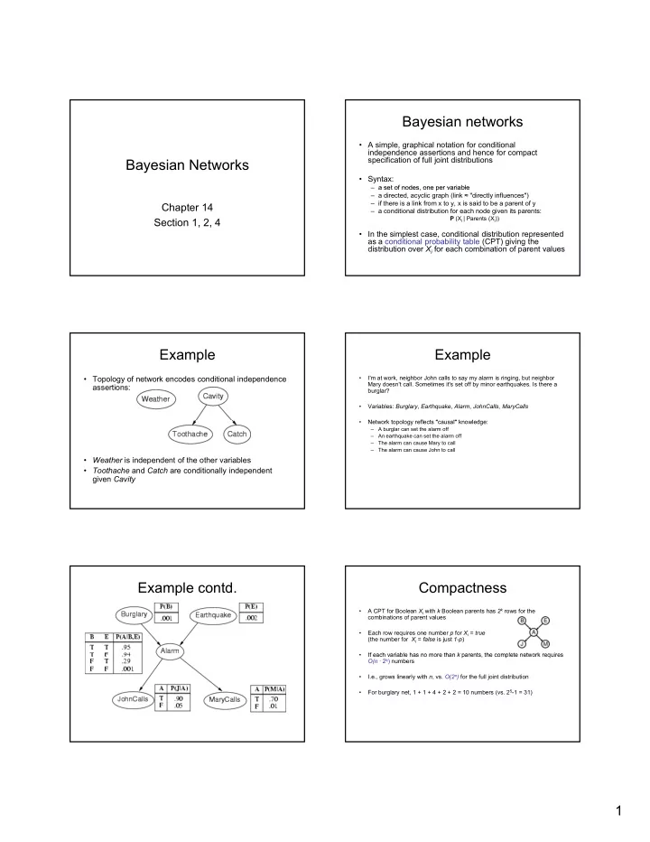Example • Topology of network encodes conditional independence • I'm at work, neighbor John calls to say my alarm is ringing, but neighbor Mary doesn't call. Sometimes it's set off by minor earthquakes. Is there a assertions: burglar? • Variables: Burglary , Earthquake , Alarm , JohnCalls , MaryCalls • Network topology reflects "causal" knowledge: Network topology reflects "causal" knowledge: – A burglar can set the alarm off – An earthquake can set the alarm off – The alarm can cause Mary to call – The alarm can cause John to call • Weather is independent of the other variables • Toothache and Catch are conditionally independent given Cavity Example contd. Compactness A CPT for Boolean X i with k Boolean parents has 2 k rows for the • combinations of parent values • Each row requires one number p for X i = true (the number for X i = false is just 1-p ) • If each variable has no more than k parents the complete network requires If each variable has no more than k parents, the complete network requires O(n · 2 k ) numbers • I.e., grows linearly with n , vs. O(2 n ) for the full joint distribution • For burglary net, 1 + 1 + 4 + 2 + 2 = 10 numbers (vs. 2 5 -1 = 31) 1

Back to the dentist example ... Semantics  We now represent the world of the The full joint distribution is defined as the product of the local conditional distributions: dentist D using three propositions – n Cavity, Toothache, and PCatch P (X 1 , … ,X n ) = π i = 1 P (X i | Parents(X i ))  D’s belief state consists of 2 3 = 8 states Thus each entry in the joint distribution is represented by the product of the appropriate elements of the conditional probability tables in each with some probability: the Bayesian network. {cavity ^ toothache ^ pcatch, e.g., P (j ^ m ^ a ^ ¬b ^ ¬ e) ¬ cavity ^ toothache ^ pcatch, = P (j | a) P (m | a) P (a | ¬ b, ¬ e) P (¬ b) P (¬ e) cavity ^ ¬ toothache ^ pcatch,...} = 0.90 * 0.70 * 0.001 * 0.999 * 0.998 = 0.00062 Probabilistic Inference The belief state is defined by the full joint probability of the propositions toothache ¬ toothache toothache ¬ toothache pcatch p ¬ pcatch p p pcatch ¬ pcatch p p pcatch ¬ pcatch pcatch p p ¬ pcatch p cavity 0.108 0.012 0.072 0.008 cavity 0.108 0.012 0.072 0.008 ¬ cavity 0.016 0.064 0.144 0.576 ¬ cavity 0.016 0.064 0.144 0.576 P(cavity  toothache) = 0.108 + 0.012 + ... = 0.28 Probabilistic Inference Probabilistic Inference toothache ¬ toothache toothache ¬ toothache pcatch p ¬ pcatch pcatch p p ¬ pcatch p pcatch p ¬ pcatch pcatch p p ¬ pcatch p cavity 0.108 0.012 0.072 0.008 cavity 0.108 0.012 0.072 0.008 ¬ cavity 0.016 0.064 0.144 0.576 ¬ cavity 0.016 0.064 0.144 0.576 Marginalization: P (c) =  t  pc P(c ^ t ^ pc) P(cavity) = 0.108 + 0.012 + 0.072 + 0.008 using the conventions that c = cavity or ¬ cavity and that = 0.2  t is the sum over t = {toothache, ¬ toothache} 2

Conditional Probability toothache ¬ toothache pcatch ¬ pcatch pcatch ¬ pcatch  P(A ^ B) = P(A|B) P(B) cavity 0.108 0.012 0.072 0.008 = P(B|A) P(A) ¬ cavity 0.016 0.064 0.144 0.576 P(A|B) is the posterior probability of A given B given B P(cavity|toothache) = P(cavity ^ toothache)/P(toothache) = (0.108+0.012)/(0.108+0.012+0.016+0.064) = 0.6 Interpretation: After observing Toothache, the patient is no longer an “average” one, and the prior probabilities of Cavity is no longer valid P(cavity|toothache) is calculated by keeping the ratios of the probabilities of the 4 cases unchanged, and normalizing their sum to 1 Conditional Probability toothache ¬ toothache pcatch ¬ pcatch pcatch ¬ pcatch  P(A ^ B) = P(A|B) P(B) cavity 0.108 0.012 0.072 0.008 = P(B|A) P(A)  P(A ^ B ^ C) = P(A|B,C) P(B ^ C) ¬ cavity 0.016 0.064 0.144 0.576 = P(A|B,C) P(B|C) P(C) P(A|B,C) P(B|C) P(C) P(cavity|toothache) = P(cavity ^ toothache)/P(toothache)  P(Cavity) =  t  pc P(Cavity ^ t ^ pc) = (0.108+0.012)/(0.108+0.012+0.016+0.064) = 0.6 P( ¬ cavity|toothache)=P( ¬ cavity ^ toothache)/P(toothache) =  t  pc P(Cavity|t,pc) P(t ^ pc) = (0.016+0.064)/(0.108+0.012+0.016+0.064) = 0.4 P(C|toochache) =  P(C ^ toothache)  P(c) =  t  pc P(c ^ t ^ pc) =   pc P(C ^ toothache ^ pc) normalization =  [(0.108, 0.016) + (0.012, 0.064)] =  t  pc P(c|t,pc)P(t ^ pc) constant =  (0.12, 0.08) = (0.6, 0.4) Independence Issues  Two random variables A and B are  If a state is described by n propositions, then a belief state contains 2 n states independent if P(A ^ B) = P(A) P(B) (possibly, some have probability 0) hence if P(A|B) = P(A) hence if P(A|B) = P(A)   Modeling difficulty: many numbers   Modeling difficulty: many numbers must be entered in the first place  Two random variables A and B are   Computational issue: memory size and independent given C, if time P(A ^ B | C) = P(A|C) P(B | C) hence if P(A|B,C) = P(A|C) 3

Bayesian Network toothache ¬ toothache pcatch ¬ pcatch pcatch ¬ pcatch Notice that Cavity is the “cause” of both Toothache  and PCatch, and represent the causality links explicitly cavity 0.108 0.012 0.072 0.008 Give the prior probability distribution of Cavity  Give the conditional probability tables of Toothache ¬ cavity 0.016 0.064 0.144 0.576  and PCatch P(cavity)  toothache and pcatch are independent given 0.2 Cavity cavity (or ¬ cavity), but this relation is hidden in the numbers ! [Verify this] P(toothache|c) P(pclass|c)  Bayesian networks explicitly represent cavity 0.6 cavity 0.9 0.02 independence among propositions to reduce ¬ cavity 0.1 ¬ cavity the number of probabilities defining a belief Toothache PCatch state 5 probabilities, instead of 7 A More Complex BN A More Complex BN P(B) P(E) Burglary Earthquake Burglary Earthquake 0.001 0.002 causes Intuitive meaning of Size of the Size of the B E P(A| … ) ( | ) arc from x to y: “x T T 0.95 Directed CPT for a has direct influence Alarm Alarm T F 0.94 acyclic graph node with k F T 0.29 on y” F F 0.001 parents: 2 k effects A P(J|…) A P(M|…) JohnCalls MaryCalls JohnCalls MaryCalls T 0.90 T 0.70 F 0.05 F 0.01 10 probabilities, instead of 31 What does the BN encode? What does the BN encode? Burglary Earthquake Burglary Earthquake Alarm Alarm A node is independent of A node is independent of A node is independent of JohnCalls MaryCalls JohnCalls its non-descendants MaryCalls given its parents Each of the beliefs The beliefs JohnCalls JohnCalls and MaryCalls is and MaryCalls are independent of Burglary independent given For instance, the reasons why For example, John does John and Mary may not call if and Earthquake given Alarm or ¬ Alarm there is an alarm are unrelated not observe any burglaries Alarm or ¬ Alarm directly 4

Conditional Independence of Markov Blanket non-descendents A node X is conditionally independent of its non-descendents (e.g., the Zijs) A node X is conditionally independent of all other nodes in the network, given its given its parents (the Uis shown in the gray area). parents, chlidren, and chlidren’s parents. Locally Structured World  A world is locally structured (or sparse) if each But does a BN represent a of its components interacts directly with belief state? relatively few other components  In a sparse world, the CPTs are small and the BN BN contains many fewer probabilities than the t i s f b biliti s th th In other words, can we compute full joint distribution the full joint distribution of the  If the # of entries in each CPT is bounded, i.e., O(1), then the # of probabilities in a BN is propositions from it? linear in n – the # of propositions – instead of 2 n for the joint distribution Burglary Earthquake Calculation of Joint Probability Alarm JohnCalls MaryCalls  P(J ^ M ^ A ^¬ B ^¬ E) P(B) P(E) Burglary Earthquake = P(J ^ M|A , ¬ B , ¬ E) * P(A ^¬ B ^¬ E) 0.001 0.002 = P(J|A , ¬ B , ¬ E) * P(M|A , ¬ B , ¬ E) * P(A ^¬ B ^¬ E) (J and M are independent given A) (J and M are independent given A) P(j ^ m ^ a ^ ¬ b ¬^ e) = ?? P(j m a b e) ?? B E P(A| … ) ( | ) T T 0.95  P(J|A , ¬ B , ¬ E) = P(J|A) Alarm T F 0.94 F T 0.29 (J and ¬ B ^¬ E are independent given A) F F 0.001  P(M|A , ¬ B , ¬ E) = P(M|A)  P(A ^¬ B ^¬ E) = P(A| ¬ B, ¬ E) * P( ¬ B| ¬ E) * P( ¬ E) A P(J|…) A P(M|…) = P(A| ¬ B, ¬ E) * P( ¬ B) * P( ¬ E) JohnCalls MaryCalls T 0.90 T 0.70 ( ¬ B and ¬ E are independent) F 0.05 F 0.01  P(J ^ M ^ A ^¬ B ^¬ E) = P(J|A)P(M|A)P(A| ¬ B, ¬ E)P( ¬ B)P( ¬ E) 5