SLIDE 1
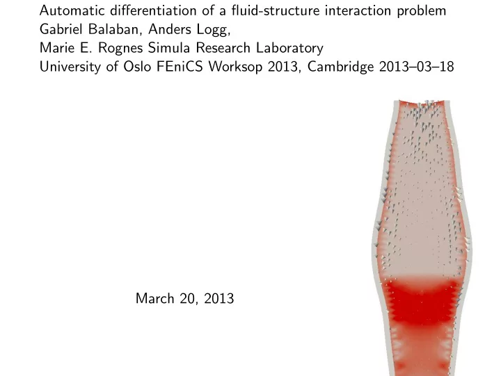
Automatic differentiation of a fluid-structure interaction problem Gabriel Balaban, Anders Logg, Marie E. Rognes Simula Research Laboratory University of Oslo FEniCS Worksop 2013, Cambridge 2013–03–18 March 20, 2013
SLIDE 2
Examples of Fluid–structure interaction
Modelling Challenges
◮ model must integrate solid and fluid mechanics ◮ fluid geometry depends on structure deformation
SLIDE 3
Solving the FSI problem
Issues:
◮ Continuum mechanics formulation ◮ Partitioned vs monolithic ◮ Fixed-pointed vs Newton ◮ Approximation of the Jacobian
In this work we:
◮ derive a Newton’s method with exact Jacobians for FSI
problems using the arbitrary Lagrangian Eulerian formulation
◮ implement a monolithic solver in Python (using FEniCS) ◮ investigate various optimizations and simplifications
SLIDE 4
Setup of the FSI problem
ΩF ωF(t) ΩS ωS(t) UF uF dS t = 0 DS
SLIDE 5
Mismatch in standard fluid and solid models
ρS ¨ DS − Div ΣS(DS) = BS ρF (˙ uF + grad uF · uF ) − div σF = bF div uF = 0
SLIDE 6
Mesh smoothing problem
Mesh equation ˙ DM − Div ΣM(DM) = 0
SLIDE 7
Arbitrary Lagrangian-Eulerian framework
u(x(X, t), t) ALE time derivative: d dt (ρu) = ˙ ρu + ρ (grad u· (u − ˙ DM)) ALE fluid equation: ρF (˙ uF + grad uF · (uF − ˙ DM)) − div σF (uF , pF ) = bF in ωF (t) div uF = 0 in ωF (t)
SLIDE 8 Interface conditions
ΓFS γFS(t)
◮ Stress continuity:
σS · n = σF · n
◮ Kinematic continuity:
uF = uS
◮ Domain continuity:
dM = dS
SLIDE 9 Linearization of the FSI problem
Two challenges:
◮ Derivative of fluid equation with respect to geometry? d dt (ρu) − div σF (uF , pF )
= bF in ωF (t) div uF = in ωF (t)
◮ Linearization of essential BCs
uF = uS
dM = dS
SLIDE 10
The reference domain approach
◮ Map the fluid problem to the reference domain ◮ Use standard techniques to differentiate ◮ Straightforward but tedious ◮ Can be automated!
SLIDE 11 Navier–Stokes pulled back to reference domain
◮ Equation:
ρF JM( ˙ UF + Grad UF · F −1
M
· (UF − ˙ DM)) − Div ΣF = BF Div (JM F −1
M
· UF ) = 0
◮ Pulled-back fluid stress:
ΣF = JM
M
+ F −⊤
M
· Grad U⊤
F ) − PF I
M
SLIDE 12 Interface conditions: How to linearize?
ΓFS γFS(t) Stress continuity: ΣS · N = ΣF · N
Kinematic continuity: UF = US
Domain continuity: DM = DS
SLIDE 13
Linearization of essential boundary conditions
Introduce Lagrange multipliers (τF , τM) and corresponding trial functions (χF , χM) Kinematic continuity: UF − USτF ΓFS + χF vF ΓFS Domain continuity: DM − DSτM ΓFS + χMvM ΓFS
SLIDE 14
The linearized FSI operator (the Jacobian)
SLIDE 15
FEniCS implementation
J = derivative(R, U)
SLIDE 16
An analytic test problem
pdf/pdf/analyticproblem.pdftex Primary variables: UF = y(1 − y) sin t PF = 2C sin t(1 − x − Cxy(1 − y)(1 − cos t)) DS = Cy(1 − y)(1 − cos t) US = Cy(1 − y) sin t DM = Cxy(1 − y)(1 − cos t)
SLIDE 17 Convergence for analytic test problem
10
10
10 mesh size hmin 10
10
10
10
10
10
10
10
L2 error 0.99 2.00 2.67
PF DS DF UF
SLIDE 18
A two-dimensional blood vessel
SLIDE 19
Break-down of run-time
Problem Routine Calls Time (s) Analytic problem Jacobian assembly 28 83.9s 90% mesh size = 231 Linear solve 28 1.86s 2% time steps = 10 Residual assembly 38 0.915s 1% Blood vessel Jacobian assembly 343 2980s 81% mesh size = 1271 Linear solve 343 254s 18% time steps = 140 Residual assembly 483 64.1s 1%
SLIDE 20 Effect of Jacobian reuse
Problem Routine Calls Analytic problem Jacobian assembly 1 (-27)
mesh size = 231 Linear solve 51 (+23)
time steps = 10 Residual assembly 61 (+23) +54% Total Runtime:
Blood vessel Jacobian assembly 25 (-308)
mesh size = 1271 Linear solve 1287 (+944)
time steps = 140 Residual assembly 1427 (+944) +192% Total
SLIDE 21 Effect of Jacobian reuse
10 20 30 40 50 60 70 time 5 10 15 20 25 30 35 Number of Iterations
Newton Iterations per time step
SLIDE 22
Optimization summary
Jacobian Reuse Jacobian Simplification Jacobian Buffering Reduced Quadrature Order Optimization Runtime Memory Robustness
SLIDE 23
Summary: How to use the automatic derivative to solve FSI problems
◮ Map the fluid equation to the
reference domain
◮ Impose essential BC’s using
Lagrange multipliers
◮ Let the automatic derivative
compute the Jacobian Challenges / work in progress:
◮ Long FFC compilation times ◮ Preconditioning