[PPT] - AutoDiff: Reverse Mode v 0 v 5 v 2 v 3 ln x 1 v 0 v 5 v 2 v 1 PowerPoint Presentation

SLIDE 1

AutoDiff: Reverse Mode

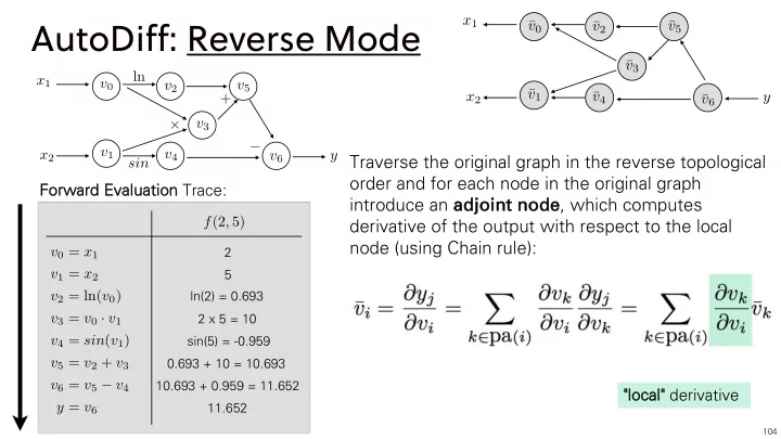
104

v0 = x1 v1 = x2 v2 = ln(v0) v3 = v0 · v1 v4 = sin(v1) v5 = v2 + v3 v6 = v5 − v4 y = v6 f(2, 5)

Forwar ard Eval valuat ation Trace:

2 5 ln(2) = 0.693 2 x 5 = 10 sin(5) = -0.959 0.693 + 10 = 10.693 10.693 + 0.959 = 11.652 11.652

+ sin +

−

ln v0 v1 v2 v4 v5 v3 v6 x1 x2 y

x1 x2 y ¯ v0 ¯ v1 ¯ v2 ¯ v3 ¯ v4 ¯ v5 ¯ v6

Traverse the original graph in the reverse topological

rder and for each node in the original graph

introduce an ad adjo join int node node, which computes derivative of the output with respect to the local node (using Chain rule):

"local cal" derivative

SLIDE 2

AutoDiff: Reverse Mode

105

v0 = x1 v1 = x2 v2 = ln(v0) v3 = v0 · v1 v4 = sin(v1) v5 = v2 + v3 v6 = v5 − v4 y = v6 f(2, 5)

Forwar ard Eval valuat ation Trace:

2 5 ln(2) = 0.693 2 x 5 = 10 sin(5) = -0.959 0.693 + 10 = 10.693 10.693 + 0.959 = 11.652 11.652

+ sin +

−

ln v0 v1 v2 v4 v5 v3 v6 x1 x2 y

Backwards Derivative ∂v3 ¯ v4 = ¯ v6 ∂v6 ∂v4 ∂v4 ¯ v5 = ¯ v6 ∂v6 ∂v5 ∂y ∂v5 ¯ v6 = ∂y ∂v6

1 1x1 = 1

= ¯ v6 · 1 = ¯ v6 · (−1)

1x-1 = -1

∂v2 ¯ v3 = ¯ v5 ∂v5 ∂v3 = ¯ v5 · (1)

1x1 = 1

∂v1 ∂v1 ¯ v2 = ¯ v5 ∂v5 ∂v2 = ¯ v5 · (1)

1x1 = 1

∂v1 ∂v0

1 = ¯

v3 ∂v3 ∂v1 + ¯ v4 ∂v4 ∂v1 ∂v ¯ v1 = ¯ = ¯ v3v0 + ¯ v4cos(v1)

1.716

= ¯ v3v1 + ¯ v2 1 v0

5.5

¯ v0 = ¯ v3 ∂v3 ∂v0 + ¯ v2 ∂v2 ∂v0

Backw ackwar ards Derivat vative ve Trace:

SLIDE 3

AutoDiff: Reverse Mode

106

v0 = x1 v1 = x2 v2 = ln(v0) v3 = v0 · v1 v4 = sin(v1) v5 = v2 + v3 v6 = v5 − v4 y = v6 f(2, 5)

Forwar ard Eval valuat ation Trace:

2 5 ln(2) = 0.693 2 x 5 = 10 sin(5) = -0.959 0.693 + 10 = 10.693 10.693 + 0.959 = 11.652 11.652

+ sin +

−

ln v0 v1 v2 v4 v5 v3 v6 x1 x2 y

Backwards Derivative ∂v3 ¯ v4 = ¯ v6 ∂v6 ∂v4 ∂v4 ¯ v5 = ¯ v6 ∂v6 ∂v5 ∂y ∂v5 ¯ v6 = ∂y ∂v6

1 1x1 = 1

= ¯ v6 · 1 = ¯ v6 · (−1)

1x-1 = -1

∂v2 ¯ v3 = ¯ v5 ∂v5 ∂v3 = ¯ v5 · (1)

1x1 = 1

∂v1 ∂v1 ¯ v2 = ¯ v5 ∂v5 ∂v2 = ¯ v5 · (1)

1x1 = 1

∂v1 ∂v0

1 = ¯

v3 ∂v3 ∂v1 + ¯ v4 ∂v4 ∂v1 ∂v ¯ v1 = ¯ = ¯ v3v0 + ¯ v4cos(v1)

1.716

= ¯ v3v1 + ¯ v2 1 v0

5.5

¯ v0 = ¯ v3 ∂v3 ∂v0 + ¯ v2 ∂v2 ∂v0

Backw ackwar ards Derivat vative ve Trace:

SLIDE 4

AutoDiff: Reverse Mode

107

v0 = x1 v1 = x2 v2 = ln(v0) v3 = v0 · v1 v4 = sin(v1) v5 = v2 + v3 v6 = v5 − v4 y = v6 f(2, 5)

Forwar ard Eval valuat ation Trace:

2 5 ln(2) = 0.693 2 x 5 = 10 sin(5) = -0.959 0.693 + 10 = 10.693 10.693 + 0.959 = 11.652 11.652

+ sin +

−

ln v0 v1 v2 v4 v5 v3 v6 x1 x2 y

Backwards Derivative ∂v3 ¯ v4 = ¯ v6 ∂v6 ∂v4 ∂v4 ¯ v5 = ¯ v6 ∂v6 ∂v5 ∂y ∂v5 ¯ v6 = ∂y ∂v6

1 1x1 = 1

= ¯ v6 · 1 = ¯ v6 · (−1)

1x-1 = -1

∂v2 ¯ v3 = ¯ v5 ∂v5 ∂v3 = ¯ v5 · (1)

1x1 = 1

∂v1 ∂v1 ¯ v2 = ¯ v5 ∂v5 ∂v2 = ¯ v5 · (1)

1x1 = 1

∂v1 ∂v0

1 = ¯

v3 ∂v3 ∂v1 + ¯ v4 ∂v4 ∂v1 ∂v ¯ v1 = ¯ = ¯ v3v0 + ¯ v4cos(v1)

1.716

= ¯ v3v1 + ¯ v2 1 v0

5.5

¯ v0 = ¯ v3 ∂v3 ∂v0 + ¯ v2 ∂v2 ∂v0

Backw ackwar ards Derivat vative ve Trace:

1

SLIDE 5

AutoDiff: Reverse Mode

108

v0 = x1 v1 = x2 v2 = ln(v0) v3 = v0 · v1 v4 = sin(v1) v5 = v2 + v3 v6 = v5 − v4 y = v6 f(2, 5)

Forwar ard Eval valuat ation Trace:

2 5 ln(2) = 0.693 2 x 5 = 10 sin(5) = -0.959 0.693 + 10 = 10.693 10.693 + 0.959 = 11.652 11.652

+ sin +

−

ln v0 v1 v2 v4 v5 v3 v6 x1 x2 y

Backwards Derivative ∂v3 ¯ v4 = ¯ v6 ∂v6 ∂v4 ∂v4 ¯ v5 = ¯ v6 ∂v6 ∂v5 ∂y ∂v5 ¯ v6 = ∂y ∂v6

1 1x1 = 1

= ¯ v6 · 1 = ¯ v6 · (−1)

1x-1 = -1

∂v2 ¯ v3 = ¯ v5 ∂v5 ∂v3 = ¯ v5 · (1)

1x1 = 1

∂v1 ∂v1 ¯ v2 = ¯ v5 ∂v5 ∂v2 = ¯ v5 · (1)

1x1 = 1

∂v1 ∂v0

1 = ¯

v3 ∂v3 ∂v1 + ¯ v4 ∂v4 ∂v1 ∂v ¯ v1 = ¯ = ¯ v3v0 + ¯ v4cos(v1)

1.716

= ¯ v3v1 + ¯ v2 1 v0

5.5

¯ v0 = ¯ v3 ∂v3 ∂v0 + ¯ v2 ∂v2 ∂v0

Backw ackwar ards Derivat vative ve Trace:

1

SLIDE 6

AutoDiff: Reverse Mode

109

v0 = x1 v1 = x2 v2 = ln(v0) v3 = v0 · v1 v4 = sin(v1) v5 = v2 + v3 v6 = v5 − v4 y = v6 f(2, 5)

Forwar ard Eval valuat ation Trace:

2 5 ln(2) = 0.693 2 x 5 = 10 sin(5) = -0.959 0.693 + 10 = 10.693 10.693 + 0.959 = 11.652 11.652

+ sin +

−

ln v0 v1 v2 v4 v5 v3 v6 x1 x2 y

Backwards Derivative ∂v3 ¯ v4 = ¯ v6 ∂v6 ∂v4 ∂v4 ¯ v5 = ¯ v6 ∂v6 ∂v5 ∂y ∂v5 ¯ v6 = ∂y ∂v6

1 1x1 = 1

= ¯ v6 · 1 = ¯ v6 · (−1)

1x-1 = -1

∂v2 ¯ v3 = ¯ v5 ∂v5 ∂v3 = ¯ v5 · (1)

1x1 = 1

∂v1 ∂v1 ¯ v2 = ¯ v5 ∂v5 ∂v2 = ¯ v5 · (1)

1x1 = 1

∂v1 ∂v0

1 = ¯

v3 ∂v3 ∂v1 + ¯ v4 ∂v4 ∂v1 ∂v ¯ v1 = ¯ = ¯ v3v0 + ¯ v4cos(v1)

1.716

= ¯ v3v1 + ¯ v2 1 v0

5.5

¯ v0 = ¯ v3 ∂v3 ∂v0 + ¯ v2 ∂v2 ∂v0

Backw ackwar ards Derivat vative ve Trace:

1

SLIDE 7

AutoDiff: Reverse Mode

110

v0 = x1 v1 = x2 v2 = ln(v0) v3 = v0 · v1 v4 = sin(v1) v5 = v2 + v3 v6 = v5 − v4 y = v6 f(2, 5)

Forwar ard Eval valuat ation Trace:

2 5 ln(2) = 0.693 2 x 5 = 10 sin(5) = -0.959 0.693 + 10 = 10.693 10.693 + 0.959 = 11.652 11.652

+ sin +

−

ln v0 v1 v2 v4 v5 v3 v6 x1 x2 y

Backwards Derivative ∂v3 ¯ v4 = ¯ v6 ∂v6 ∂v4 ∂v4 ¯ v5 = ¯ v6 ∂v6 ∂v5 ∂y ∂v5 ¯ v6 = ∂y ∂v6

1 1x1 = 1

= ¯ v6 · 1 = ¯ v6 · (−1)

1x-1 = -1

∂v2 ¯ v3 = ¯ v5 ∂v5 ∂v3 = ¯ v5 · (1)

1x1 = 1

∂v1 ∂v1 ¯ v2 = ¯ v5 ∂v5 ∂v2 = ¯ v5 · (1)

1x1 = 1

∂v1 ∂v0

1 = ¯

v3 ∂v3 ∂v1 + ¯ v4 ∂v4 ∂v1 ∂v ¯ v1 = ¯ = ¯ v3v0 + ¯ v4cos(v1)

1.716

= ¯ v3v1 + ¯ v2 1 v0

5.5

¯ v0 = ¯ v3 ∂v3 ∂v0 + ¯ v2 ∂v2 ∂v0

Backw ackwar ards Derivat vative ve Trace:

1

SLIDE 8

AutoDiff: Reverse Mode

111

v0 = x1 v1 = x2 v2 = ln(v0) v3 = v0 · v1 v4 = sin(v1) v5 = v2 + v3 v6 = v5 − v4 y = v6 f(2, 5)

Forwar ard Eval valuat ation Trace:

2 5 ln(2) = 0.693 2 x 5 = 10 sin(5) = -0.959 0.693 + 10 = 10.693 10.693 + 0.959 = 11.652 11.652

+ sin +

−

ln v0 v1 v2 v4 v5 v3 v6 x1 x2 y

Backwards Derivative ∂v3 ¯ v4 = ¯ v6 ∂v6 ∂v4 ∂v4 ¯ v5 = ¯ v6 ∂v6 ∂v5 ∂y ∂v5 ¯ v6 = ∂y ∂v6

1 1x1 = 1

= ¯ v6 · 1 = ¯ v6 · (−1)

1x-1 = -1

∂v2 ¯ v3 = ¯ v5 ∂v5 ∂v3 = ¯ v5 · (1)

1x1 = 1

∂v1 ∂v1 ¯ v2 = ¯ v5 ∂v5 ∂v2 = ¯ v5 · (1)

1x1 = 1

∂v1 ∂v0

1 = ¯

v3 ∂v3 ∂v1 + ¯ v4 ∂v4 ∂v1 ∂v ¯ v1 = ¯ = ¯ v3v0 + ¯ v4cos(v1)

1.716

= ¯ v3v1 + ¯ v2 1 v0

5.5

¯ v0 = ¯ v3 ∂v3 ∂v0 + ¯ v2 ∂v2 ∂v0

Backw ackwar ards Derivat vative ve Trace:

1 1x1 = 1

SLIDE 9

AutoDiff: Reverse Mode

112

v0 = x1 v1 = x2 v2 = ln(v0) v3 = v0 · v1 v4 = sin(v1) v5 = v2 + v3 v6 = v5 − v4 y = v6 f(2, 5)

Forwar ard Eval valuat ation Trace:

2 5 ln(2) = 0.693 2 x 5 = 10 sin(5) = -0.959 0.693 + 10 = 10.693 10.693 + 0.959 = 11.652 11.652

+ sin +

−

ln v0 v1 v2 v4 v5 v3 v6 x1 x2 y

Backwards Derivative ∂v3 ¯ v4 = ¯ v6 ∂v6 ∂v4 ∂v4 ¯ v5 = ¯ v6 ∂v6 ∂v5 ∂y ∂v5 ¯ v6 = ∂y ∂v6

1 1x1 = 1

= ¯ v6 · 1 = ¯ v6 · (−1)

1x-1 = -1

∂v2 ¯ v3 = ¯ v5 ∂v5 ∂v3 = ¯ v5 · (1)

1x1 = 1

∂v1 ∂v1 ¯ v2 = ¯ v5 ∂v5 ∂v2 = ¯ v5 · (1)

1x1 = 1

∂v1 ∂v0

1 = ¯

v3 ∂v3 ∂v1 + ¯ v4 ∂v4 ∂v1 ∂v ¯ v1 = ¯ = ¯ v3v0 + ¯ v4cos(v1)

1.716

= ¯ v3v1 + ¯ v2 1 v0

5.5

¯ v0 = ¯ v3 ∂v3 ∂v0 + ¯ v2 ∂v2 ∂v0

Backw ackwar ards Derivat vative ve Trace:

1 1x1 = 1

SLIDE 10

AutoDiff: Reverse Mode

113

v0 = x1 v1 = x2 v2 = ln(v0) v3 = v0 · v1 v4 = sin(v1) v5 = v2 + v3 v6 = v5 − v4 y = v6 f(2, 5)

Forwar ard Eval valuat ation Trace:

2 5 ln(2) = 0.693 2 x 5 = 10 sin(5) = -0.959 0.693 + 10 = 10.693 10.693 + 0.959 = 11.652 11.652

+ sin +

−

ln v0 v1 v2 v4 v5 v3 v6 x1 x2 y

Backwards Derivative ∂v3 ¯ v4 = ¯ v6 ∂v6 ∂v4 ∂v4 ¯ v5 = ¯ v6 ∂v6 ∂v5 ∂y ∂v5 ¯ v6 = ∂y ∂v6

1 1x1 = 1

= ¯ v6 · 1 = ¯ v6 · (−1)

1x-1 = -1

∂v2 ¯ v3 = ¯ v5 ∂v5 ∂v3 = ¯ v5 · (1)

1x1 = 1

∂v1 ∂v1 ¯ v2 = ¯ v5 ∂v5 ∂v2 = ¯ v5 · (1)

1x1 = 1

∂v1 ∂v0

1 = ¯

v3 ∂v3 ∂v1 + ¯ v4 ∂v4 ∂v1 ∂v ¯ v1 = ¯ = ¯ v3v0 + ¯ v4cos(v1)

1.716

= ¯ v3v1 + ¯ v2 1 v0

5.5

¯ v0 = ¯ v3 ∂v3 ∂v0 + ¯ v2 ∂v2 ∂v0

Backw ackwar ards Derivat vative ve Trace:

1 1x1 = 1

SLIDE 11

AutoDiff: Reverse Mode

114

v0 = x1 v1 = x2 v2 = ln(v0) v3 = v0 · v1 v4 = sin(v1) v5 = v2 + v3 v6 = v5 − v4 y = v6 f(2, 5)

Forwar ard Eval valuat ation Trace:

2 5 ln(2) = 0.693 2 x 5 = 10 sin(5) = -0.959 0.693 + 10 = 10.693 10.693 + 0.959 = 11.652 11.652

+ sin +

−

ln v0 v1 v2 v4 v5 v3 v6 x1 x2 y

Backwards Derivative ∂v3 ¯ v4 = ¯ v6 ∂v6 ∂v4 ∂v4 ¯ v5 = ¯ v6 ∂v6 ∂v5 ∂y ∂v5 ¯ v6 = ∂y ∂v6

1 1x1 = 1

= ¯ v6 · 1 = ¯ v6 · (−1)

1x-1 = -1

∂v2 ¯ v3 = ¯ v5 ∂v5 ∂v3 = ¯ v5 · (1)

1x1 = 1

∂v1 ∂v1 ¯ v2 = ¯ v5 ∂v5 ∂v2 = ¯ v5 · (1)

1x1 = 1

∂v1 ∂v0

1 = ¯

v3 ∂v3 ∂v1 + ¯ v4 ∂v4 ∂v1 ∂v ¯ v1 = ¯ = ¯ v3v0 + ¯ v4cos(v1)

1.716

= ¯ v3v1 + ¯ v2 1 v0

5.5

¯ v0 = ¯ v3 ∂v3 ∂v0 + ¯ v2 ∂v2 ∂v0

Backw ackwar ards Derivat vative ve Trace:

1 1x1 = 1

SLIDE 12

AutoDiff: Reverse Mode

115

v0 = x1 v1 = x2 v2 = ln(v0) v3 = v0 · v1 v4 = sin(v1) v5 = v2 + v3 v6 = v5 − v4 y = v6 f(2, 5)

Forwar ard Eval valuat ation Trace:

2 5 ln(2) = 0.693 2 x 5 = 10 sin(5) = -0.959 0.693 + 10 = 10.693 10.693 + 0.959 = 11.652 11.652

+ sin +

−

ln v0 v1 v2 v4 v5 v3 v6 x1 x2 y

Backwards Derivative ∂v3 ¯ v4 = ¯ v6 ∂v6 ∂v4 ∂v4 ¯ v5 = ¯ v6 ∂v6 ∂v5 ∂y ∂v5 ¯ v6 = ∂y ∂v6

1 1x1 = 1

= ¯ v6 · 1 = ¯ v6 · (−1)

1x-1 = -1

∂v2 ¯ v3 = ¯ v5 ∂v5 ∂v3 = ¯ v5 · (1)

1x1 = 1

∂v1 ∂v1 ¯ v2 = ¯ v5 ∂v5 ∂v2 = ¯ v5 · (1)

1x1 = 1

∂v1 ∂v0

1 = ¯

v3 ∂v3 ∂v1 + ¯ v4 ∂v4 ∂v1 ∂v ¯ v1 = ¯ = ¯ v3v0 + ¯ v4cos(v1)

1.716

= ¯ v3v1 + ¯ v2 1 v0

5.5

¯ v0 = ¯ v3 ∂v3 ∂v0 + ¯ v2 ∂v2 ∂v0

Backw ackwar ards Derivat vative ve Trace:

1 1x1 = 1 1x-1 = -1

SLIDE 13

AutoDiff: Reverse Mode

116

v0 = x1 v1 = x2 v2 = ln(v0) v3 = v0 · v1 v4 = sin(v1) v5 = v2 + v3 v6 = v5 − v4 y = v6 f(2, 5)

Forwar ard Eval valuat ation Trace:

2 5 ln(2) = 0.693 2 x 5 = 10 sin(5) = -0.959 0.693 + 10 = 10.693 10.693 + 0.959 = 11.652 11.652

+ sin +

−

ln v0 v1 v2 v4 v5 v3 v6 x1 x2 y

Backwards Derivative ∂v3 ¯ v4 = ¯ v6 ∂v6 ∂v4 ∂v4 ¯ v5 = ¯ v6 ∂v6 ∂v5 ∂y ∂v5 ¯ v6 = ∂y ∂v6

1 1x1 = 1

= ¯ v6 · 1 = ¯ v6 · (−1)

1x-1 = -1

∂v2 ¯ v3 = ¯ v5 ∂v5 ∂v3 = ¯ v5 · (1)

1x1 = 1

∂v1 ∂v1 ¯ v2 = ¯ v5 ∂v5 ∂v2 = ¯ v5 · (1)

1x1 = 1

∂v1 ∂v0

1 = ¯

v3 ∂v3 ∂v1 + ¯ v4 ∂v4 ∂v1 ∂v ¯ v1 = ¯ = ¯ v3v0 + ¯ v4cos(v1)

1.716

= ¯ v3v1 + ¯ v2 1 v0

5.5

¯ v0 = ¯ v3 ∂v3 ∂v0 + ¯ v2 ∂v2 ∂v0

Backw ackwar ards Derivat vative ve Trace:

1 1x1 = 1 1x-1 = -1

SLIDE 14

AutoDiff: Reverse Mode

117

v0 = x1 v1 = x2 v2 = ln(v0) v3 = v0 · v1 v4 = sin(v1) v5 = v2 + v3 v6 = v5 − v4 y = v6 f(2, 5)

Forwar ard Eval valuat ation Trace:

2 5 ln(2) = 0.693 2 x 5 = 10 sin(5) = -0.959 0.693 + 10 = 10.693 10.693 + 0.959 = 11.652 11.652

+ sin +

−

ln v0 v1 v2 v4 v5 v3 v6 x1 x2 y

Backwards Derivative ∂v3 ¯ v4 = ¯ v6 ∂v6 ∂v4 ∂v4 ¯ v5 = ¯ v6 ∂v6 ∂v5 ∂y ∂v5 ¯ v6 = ∂y ∂v6

1 1x1 = 1

= ¯ v6 · 1 = ¯ v6 · (−1)

1x-1 = -1

∂v2 ¯ v3 = ¯ v5 ∂v5 ∂v3 = ¯ v5 · (1)

1x1 = 1

∂v1 ∂v1 ¯ v2 = ¯ v5 ∂v5 ∂v2 = ¯ v5 · (1)

1x1 = 1

∂v1 ∂v0

1 = ¯

v3 ∂v3 ∂v1 + ¯ v4 ∂v4 ∂v1 ∂v ¯ v1 = ¯ = ¯ v3v0 + ¯ v4cos(v1)

1.716

= ¯ v3v1 + ¯ v2 1 v0

5.5

¯ v0 = ¯ v3 ∂v3 ∂v0 + ¯ v2 ∂v2 ∂v0

Backw ackwar ards Derivat vative ve Trace:

1 1x1 = 1 1x-1 = -1

SLIDE 15

AutoDiff: Reverse Mode

118

v0 = x1 v1 = x2 v2 = ln(v0) v3 = v0 · v1 v4 = sin(v1) v5 = v2 + v3 v6 = v5 − v4 y = v6 f(2, 5)

Forwar ard Eval valuat ation Trace:

2 5 ln(2) = 0.693 2 x 5 = 10 sin(5) = -0.959 0.693 + 10 = 10.693 10.693 + 0.959 = 11.652 11.652

+ sin +

−

ln v0 v1 v2 v4 v5 v3 v6 x1 x2 y

Backwards Derivative ∂v3 ¯ v4 = ¯ v6 ∂v6 ∂v4 ∂v4 ¯ v5 = ¯ v6 ∂v6 ∂v5 ∂y ∂v5 ¯ v6 = ∂y ∂v6

1 1x1 = 1

= ¯ v6 · 1 = ¯ v6 · (−1)

1x-1 = -1

∂v2 ¯ v3 = ¯ v5 ∂v5 ∂v3 = ¯ v5 · (1)

1x1 = 1

∂v1 ∂v1 ¯ v2 = ¯ v5 ∂v5 ∂v2 = ¯ v5 · (1)

1x1 = 1

∂v1 ∂v0

1 = ¯

v3 ∂v3 ∂v1 + ¯ v4 ∂v4 ∂v1 ∂v ¯ v1 = ¯ = ¯ v3v0 + ¯ v4cos(v1)

1.716

= ¯ v3v1 + ¯ v2 1 v0

5.5

¯ v0 = ¯ v3 ∂v3 ∂v0 + ¯ v2 ∂v2 ∂v0

Backw ackwar ards Derivat vative ve Trace:

1 1x1 = 1 1x-1 = -1

SLIDE 16

AutoDiff: Reverse Mode

119

v0 = x1 v1 = x2 v2 = ln(v0) v3 = v0 · v1 v4 = sin(v1) v5 = v2 + v3 v6 = v5 − v4 y = v6 f(2, 5)

Forwar ard Eval valuat ation Trace:

2 5 ln(2) = 0.693 2 x 5 = 10 sin(5) = -0.959 0.693 + 10 = 10.693 10.693 + 0.959 = 11.652 11.652

+ sin +

−

ln v0 v1 v2 v4 v5 v3 v6 x1 x2 y

Backwards Derivative ∂v3 ¯ v4 = ¯ v6 ∂v6 ∂v4 ∂v4 ¯ v5 = ¯ v6 ∂v6 ∂v5 ∂y ∂v5 ¯ v6 = ∂y ∂v6

1 1x1 = 1

= ¯ v6 · 1 = ¯ v6 · (−1)

1x-1 = -1

∂v2 ¯ v3 = ¯ v5 ∂v5 ∂v3 = ¯ v5 · (1)

1x1 = 1

∂v1 ∂v1 ¯ v2 = ¯ v5 ∂v5 ∂v2 = ¯ v5 · (1)

1x1 = 1

∂v1 ∂v0

1 = ¯

v3 ∂v3 ∂v1 + ¯ v4 ∂v4 ∂v1 ∂v ¯ v1 = ¯ = ¯ v3v0 + ¯ v4cos(v1)

1.716

= ¯ v3v1 + ¯ v2 1 v0

5.5

¯ v0 = ¯ v3 ∂v3 ∂v0 + ¯ v2 ∂v2 ∂v0

Backw ackwar ards Derivat vative ve Trace:

1 1x1 = 1 1x-1 = -1 1x1 = 1

SLIDE 17

AutoDiff: Reverse Mode

120

v0 = x1 v1 = x2 v2 = ln(v0) v3 = v0 · v1 v4 = sin(v1) v5 = v2 + v3 v6 = v5 − v4 y = v6 f(2, 5)

Forwar ard Eval valuat ation Trace:

2 5 ln(2) = 0.693 2 x 5 = 10 sin(5) = -0.959 0.693 + 10 = 10.693 10.693 + 0.959 = 11.652 11.652

+ sin +

−

ln v0 v1 v2 v4 v5 v3 v6 x1 x2 y

Backwards Derivative ∂v3 ¯ v4 = ¯ v6 ∂v6 ∂v4 ∂v4 ¯ v5 = ¯ v6 ∂v6 ∂v5 ∂y ∂v5 ¯ v6 = ∂y ∂v6

1 1x1 = 1

= ¯ v6 · 1 = ¯ v6 · (−1)

1x-1 = -1

∂v2 ¯ v3 = ¯ v5 ∂v5 ∂v3 = ¯ v5 · (1)

1x1 = 1

∂v1 ∂v1 ¯ v2 = ¯ v5 ∂v5 ∂v2 = ¯ v5 · (1)

1x1 = 1

∂v1 ∂v0

1 = ¯

v3 ∂v3 ∂v1 + ¯ v4 ∂v4 ∂v1 ∂v ¯ v1 = ¯ = ¯ v3v0 + ¯ v4cos(v1)

1.716

= ¯ v3v1 + ¯ v2 1 v0

5.5

¯ v0 = ¯ v3 ∂v3 ∂v0 + ¯ v2 ∂v2 ∂v0

Backw ackwar ards Derivat vative ve Trace:

1 1x1 = 1 1x-1 = -1 1x1 = 1

SLIDE 18

AutoDiff: Reverse Mode

121

v0 = x1 v1 = x2 v2 = ln(v0) v3 = v0 · v1 v4 = sin(v1) v5 = v2 + v3 v6 = v5 − v4 y = v6 f(2, 5)

Forwar ard Eval valuat ation Trace:

2 5 ln(2) = 0.693 2 x 5 = 10 sin(5) = -0.959 0.693 + 10 = 10.693 10.693 + 0.959 = 11.652 11.652

+ sin +

−

ln v0 v1 v2 v4 v5 v3 v6 x1 x2 y

Backwards Derivative ∂v3 ¯ v4 = ¯ v6 ∂v6 ∂v4 ∂v4 ¯ v5 = ¯ v6 ∂v6 ∂v5 ∂y ∂v5 ¯ v6 = ∂y ∂v6

1 1x1 = 1

= ¯ v6 · 1 = ¯ v6 · (−1)

1x-1 = -1

∂v2 ¯ v3 = ¯ v5 ∂v5 ∂v3 = ¯ v5 · (1)

1x1 = 1

∂v1 ∂v1 ¯ v2 = ¯ v5 ∂v5 ∂v2 = ¯ v5 · (1)

1x1 = 1

∂v1 ∂v0

1 = ¯

v3 ∂v3 ∂v1 + ¯ v4 ∂v4 ∂v1 ∂v ¯ v1 = ¯ = ¯ v3v0 + ¯ v4cos(v1)

1.716

= ¯ v3v1 + ¯ v2 1 v0

5.5

¯ v0 = ¯ v3 ∂v3 ∂v0 + ¯ v2 ∂v2 ∂v0

Backw ackwar ards Derivat vative ve Trace:

1 1x1 = 1 1x-1 = -1 1x1 = 1

SLIDE 19

AutoDiff: Reverse Mode

122

v0 = x1 v1 = x2 v2 = ln(v0) v3 = v0 · v1 v4 = sin(v1) v5 = v2 + v3 v6 = v5 − v4 y = v6 f(2, 5)

Forwar ard Eval valuat ation Trace:

2 5 ln(2) = 0.693 2 x 5 = 10 sin(5) = -0.959 0.693 + 10 = 10.693 10.693 + 0.959 = 11.652 11.652

+ sin +

−

ln v0 v1 v2 v4 v5 v3 v6 x1 x2 y

Backwards Derivative ∂v3 ¯ v4 = ¯ v6 ∂v6 ∂v4 ∂v4 ¯ v5 = ¯ v6 ∂v6 ∂v5 ∂y ∂v5 ¯ v6 = ∂y ∂v6

1 1x1 = 1

= ¯ v6 · 1 = ¯ v6 · (−1)

1x-1 = -1

∂v2 ¯ v3 = ¯ v5 ∂v5 ∂v3 = ¯ v5 · (1)

1x1 = 1

∂v1 ∂v1 ¯ v2 = ¯ v5 ∂v5 ∂v2 = ¯ v5 · (1)

1x1 = 1

∂v1 ∂v0

1 = ¯

v3 ∂v3 ∂v1 + ¯ v4 ∂v4 ∂v1 ∂v ¯ v1 = ¯ = ¯ v3v0 + ¯ v4cos(v1)

1.716

= ¯ v3v1 + ¯ v2 1 v0

5.5

¯ v0 = ¯ v3 ∂v3 ∂v0 + ¯ v2 ∂v2 ∂v0

Backw ackwar ards Derivat vative ve Trace:

1 1x1 = 1 1x-1 = -1 1x1 = 1

SLIDE 20

AutoDiff: Reverse Mode

123

v0 = x1 v1 = x2 v2 = ln(v0) v3 = v0 · v1 v4 = sin(v1) v5 = v2 + v3 v6 = v5 − v4 y = v6 f(2, 5)

Forwar ard Eval valuat ation Trace:

2 5 ln(2) = 0.693 2 x 5 = 10 sin(5) = -0.959 0.693 + 10 = 10.693 10.693 + 0.959 = 11.652 11.652

+ sin +

−

ln v0 v1 v2 v4 v5 v3 v6 x1 x2 y

Backwards Derivative ∂v3 ¯ v4 = ¯ v6 ∂v6 ∂v4 ∂v4 ¯ v5 = ¯ v6 ∂v6 ∂v5 ∂y ∂v5 ¯ v6 = ∂y ∂v6

1 1x1 = 1

= ¯ v6 · 1 = ¯ v6 · (−1)

1x-1 = -1

∂v2 ¯ v3 = ¯ v5 ∂v5 ∂v3 = ¯ v5 · (1)

1x1 = 1

∂v1 ∂v1 ¯ v2 = ¯ v5 ∂v5 ∂v2 = ¯ v5 · (1)

1x1 = 1

∂v1 ∂v0

1 = ¯

v3 ∂v3 ∂v1 + ¯ v4 ∂v4 ∂v1 ∂v ¯ v1 = ¯ = ¯ v3v0 + ¯ v4cos(v1)

1.716

= ¯ v3v1 + ¯ v2 1 v0

5.5

¯ v0 = ¯ v3 ∂v3 ∂v0 + ¯ v2 ∂v2 ∂v0

Backw ackwar ards Derivat vative ve Trace:

1 1x1 = 1 1x-1 = -1 1x1 = 1 1x1 = 1

SLIDE 21

AutoDiff: Reverse Mode

124

v0 = x1 v1 = x2 v2 = ln(v0) v3 = v0 · v1 v4 = sin(v1) v5 = v2 + v3 v6 = v5 − v4 y = v6 f(2, 5)

Forwar ard Eval valuat ation Trace:

2 5 ln(2) = 0.693 2 x 5 = 10 sin(5) = -0.959 0.693 + 10 = 10.693 10.693 + 0.959 = 11.652 11.652

+ sin +

−

ln v0 v1 v2 v4 v5 v3 v6 x1 x2 y

Backwards Derivative ∂v3 ¯ v4 = ¯ v6 ∂v6 ∂v4 ∂v4 ¯ v5 = ¯ v6 ∂v6 ∂v5 ∂y ∂v5 ¯ v6 = ∂y ∂v6

1 1x1 = 1

= ¯ v6 · 1 = ¯ v6 · (−1)

1x-1 = -1

∂v2 ¯ v3 = ¯ v5 ∂v5 ∂v3 = ¯ v5 · (1)

1x1 = 1

∂v1 ∂v1 ¯ v2 = ¯ v5 ∂v5 ∂v2 = ¯ v5 · (1)

1x1 = 1

∂v1 ∂v0

1 = ¯

v3 ∂v3 ∂v1 + ¯ v4 ∂v4 ∂v1 ∂v ¯ v1 = ¯ = ¯ v3v0 + ¯ v4cos(v1)

1.716

= ¯ v3v1 + ¯ v2 1 v0

5.5

¯ v0 = ¯ v3 ∂v3 ∂v0 + ¯ v2 ∂v2 ∂v0

Backw ackwar ards Derivat vative ve Trace:

1 1x1 = 1 1x-1 = -1 1x1 = 1 1x1 = 1

SLIDE 22

AutoDiff: Reverse Mode

125

v0 = x1 v1 = x2 v2 = ln(v0) v3 = v0 · v1 v4 = sin(v1) v5 = v2 + v3 v6 = v5 − v4 y = v6 f(2, 5)

Forwar ard Eval valuat ation Trace:

2 5 ln(2) = 0.693 2 x 5 = 10 sin(5) = -0.959 0.693 + 10 = 10.693 10.693 + 0.959 = 11.652 11.652

+ sin +

−

ln v0 v1 v2 v4 v5 v3 v6 x1 x2 y

Backwards Derivative ∂v3 ¯ v4 = ¯ v6 ∂v6 ∂v4 ∂v4 ¯ v5 = ¯ v6 ∂v6 ∂v5 ∂y ∂v5 ¯ v6 = ∂y ∂v6

1 1x1 = 1

= ¯ v6 · 1 = ¯ v6 · (−1)

1x-1 = -1

∂v2 ¯ v3 = ¯ v5 ∂v5 ∂v3 = ¯ v5 · (1)

1x1 = 1

∂v1 ∂v1 ¯ v2 = ¯ v5 ∂v5 ∂v2 = ¯ v5 · (1)

1x1 = 1

∂v1 ∂v0

1 = ¯

v3 ∂v3 ∂v1 + ¯ v4 ∂v4 ∂v1 ∂v ¯ v1 = ¯ = ¯ v3v0 + ¯ v4cos(v1)

1.716

= ¯ v3v1 + ¯ v2 1 v0

5.5

¯ v0 = ¯ v3 ∂v3 ∂v0 + ¯ v2 ∂v2 ∂v0

Backw ackwar ards Derivat vative ve Trace:

1 1x1 = 1 1x-1 = -1 1x1 = 1 1x1 = 1

SLIDE 23

AutoDiff: Reverse Mode

126

v0 = x1 v1 = x2 v2 = ln(v0) v3 = v0 · v1 v4 = sin(v1) v5 = v2 + v3 v6 = v5 − v4 y = v6 f(2, 5)

Forwar ard Eval valuat ation Trace:

2 5 ln(2) = 0.693 2 x 5 = 10 sin(5) = -0.959 0.693 + 10 = 10.693 10.693 + 0.959 = 11.652 11.652

+ sin +

−

ln v0 v1 v2 v4 v5 v3 v6 x1 x2 y

Backwards Derivative ∂v3 ¯ v4 = ¯ v6 ∂v6 ∂v4 ∂v4 ¯ v5 = ¯ v6 ∂v6 ∂v5 ∂y ∂v5 ¯ v6 = ∂y ∂v6

1 1x1 = 1

= ¯ v6 · 1 = ¯ v6 · (−1)

1x-1 = -1

∂v2 ¯ v3 = ¯ v5 ∂v5 ∂v3 = ¯ v5 · (1)

1x1 = 1

∂v1 ∂v1 ¯ v2 = ¯ v5 ∂v5 ∂v2 = ¯ v5 · (1)

1x1 = 1

∂v1 ∂v0

1 = ¯

v3 ∂v3 ∂v1 + ¯ v4 ∂v4 ∂v1 ∂v ¯ v1 = ¯ = ¯ v3v0 + ¯ v4cos(v1)

1.716

= ¯ v3v1 + ¯ v2 1 v0

5.5

¯ v0 = ¯ v3 ∂v3 ∂v0 + ¯ v2 ∂v2 ∂v0

Backw ackwar ards Derivat vative ve Trace:

1 1x1 = 1 1x-1 = -1 1x1 = 1 1x1 = 1

SLIDE 24

AutoDiff: Reverse Mode

127

v0 = x1 v1 = x2 v2 = ln(v0) v3 = v0 · v1 v4 = sin(v1) v5 = v2 + v3 v6 = v5 − v4 y = v6 f(2, 5)

Forwar ard Eval valuat ation Trace:

2 5 ln(2) = 0.693 2 x 5 = 10 sin(5) = -0.959 0.693 + 10 = 10.693 10.693 + 0.959 = 11.652 11.652

+ sin +

−

ln v0 v1 v2 v4 v5 v3 v6 x1 x2 y

Backwards Derivative ∂v3 ¯ v4 = ¯ v6 ∂v6 ∂v4 ∂v4 ¯ v5 = ¯ v6 ∂v6 ∂v5 ∂y ∂v5 ¯ v6 = ∂y ∂v6

1 1x1 = 1

= ¯ v6 · 1 = ¯ v6 · (−1)

1x-1 = -1

∂v2 ¯ v3 = ¯ v5 ∂v5 ∂v3 = ¯ v5 · (1)

1x1 = 1

∂v1 ∂v1 ¯ v2 = ¯ v5 ∂v5 ∂v2 = ¯ v5 · (1)

1x1 = 1

∂v1 ∂v0

1 = ¯

v3 ∂v3 ∂v1 + ¯ v4 ∂v4 ∂v1 ∂v ¯ v1 = ¯ = ¯ v3v0 + ¯ v4cos(v1)

1.716

= ¯ v3v1 + ¯ v2 1 v0

5.5

¯ v0 = ¯ v3 ∂v3 ∂v0 + ¯ v2 ∂v2 ∂v0

Backw ackwar ards Derivat vative ve Trace:

1 1x1 = 1 1x-1 = -1 1x1 = 1 1x1 = 1

SLIDE 25

AutoDiff: Reverse Mode

128

v0 = x1 v1 = x2 v2 = ln(v0) v3 = v0 · v1 v4 = sin(v1) v5 = v2 + v3 v6 = v5 − v4 y = v6 f(2, 5)

Forwar ard Eval valuat ation Trace:

2 5 ln(2) = 0.693 2 x 5 = 10 sin(5) = -0.959 0.693 + 10 = 10.693 10.693 + 0.959 = 11.652 11.652

+ sin +

−

ln v0 v1 v2 v4 v5 v3 v6 x1 x2 y

Backwards Derivative ∂v3 ¯ v4 = ¯ v6 ∂v6 ∂v4 ∂v4 ¯ v5 = ¯ v6 ∂v6 ∂v5 ∂y ∂v5 ¯ v6 = ∂y ∂v6

1 1x1 = 1

= ¯ v6 · 1 = ¯ v6 · (−1)

1x-1 = -1

∂v2 ¯ v3 = ¯ v5 ∂v5 ∂v3 = ¯ v5 · (1)

1x1 = 1

∂v1 ∂v1 ¯ v2 = ¯ v5 ∂v5 ∂v2 = ¯ v5 · (1)

1x1 = 1

∂v1 ∂v0

1 = ¯

v3 ∂v3 ∂v1 + ¯ v4 ∂v4 ∂v1 ∂v ¯ v1 = ¯ = ¯ v3v0 + ¯ v4cos(v1)

1.716

= ¯ v3v1 + ¯ v2 1 v0

5.5

¯ v0 = ¯ v3 ∂v3 ∂v0 + ¯ v2 ∂v2 ∂v0

Backw ackwar ards Derivat vative ve Trace:

1 1x1 = 1 1x-1 = -1 1x1 = 1 1x1 = 1 1.716

SLIDE 26

AutoDiff: Reverse Mode

129

v0 = x1 v1 = x2 v2 = ln(v0) v3 = v0 · v1 v4 = sin(v1) v5 = v2 + v3 v6 = v5 − v4 y = v6 f(2, 5)

Forwar ard Eval valuat ation Trace:

2 5 ln(2) = 0.693 2 x 5 = 10 sin(5) = -0.959 0.693 + 10 = 10.693 10.693 + 0.959 = 11.652 11.652

+ sin +

−

ln v0 v1 v2 v4 v5 v3 v6 x1 x2 y

Backwards Derivative ∂v3 ¯ v4 = ¯ v6 ∂v6 ∂v4 ∂v4 ¯ v5 = ¯ v6 ∂v6 ∂v5 ∂y ∂v5 ¯ v6 = ∂y ∂v6

1 1x1 = 1

= ¯ v6 · 1 = ¯ v6 · (−1)

1x-1 = -1

∂v2 ¯ v3 = ¯ v5 ∂v5 ∂v3 = ¯ v5 · (1)

1x1 = 1

∂v1 ∂v1 ¯ v2 = ¯ v5 ∂v5 ∂v2 = ¯ v5 · (1)

1x1 = 1

∂v1 ∂v0

1 = ¯

v3 ∂v3 ∂v1 + ¯ v4 ∂v4 ∂v1 ∂v ¯ v1 = ¯ = ¯ v3v0 + ¯ v4cos(v1)

1.716

= ¯ v3v1 + ¯ v2 1 v0

5.5

¯ v0 = ¯ v3 ∂v3 ∂v0 + ¯ v2 ∂v2 ∂v0

Backw ackwar ards Derivat vative ve Trace:

1 1x1 = 1 1x-1 = -1 1x1 = 1 1x1 = 1 1.716 5.5

SLIDE 27

AutoDiff: Reverse Mode

130

v0 = x1 v1 = x2 v2 = ln(v0) v3 = v0 · v1 v4 = sin(v1) v5 = v2 + v3 v6 = v5 − v4 y = v6 f(2, 5)

Forwar ard Eval valuat ation Trace:

2 5 ln(2) = 0.693 2 x 5 = 10 sin(5) = -0.959 0.693 + 10 = 10.693 10.693 + 0.959 = 11.652 11.652

+ sin +

−

ln v0 v1 v2 v4 v5 v3 v6 x1 x2 y

Backwards Derivative ∂v3 ¯ v4 = ¯ v6 ∂v6 ∂v4 ∂v4 ¯ v5 = ¯ v6 ∂v6 ∂v5 ∂y ∂v5 ¯ v6 = ∂y ∂v6

1 1x1 = 1

= ¯ v6 · 1 = ¯ v6 · (−1)

1x-1 = -1

∂v2 ¯ v3 = ¯ v5 ∂v5 ∂v3 = ¯ v5 · (1)

1x1 = 1

∂v1 ∂v1 ¯ v2 = ¯ v5 ∂v5 ∂v2 = ¯ v5 · (1)

1x1 = 1

∂v1 ∂v0

1 = ¯

v3 ∂v3 ∂v1 + ¯ v4 ∂v4 ∂v1 ∂v ¯ v1 = ¯ = ¯ v3v0 + ¯ v4cos(v1)

1.716

= ¯ v3v1 + ¯ v2 1 v0

5.5

¯ v0 = ¯ v3 ∂v3 ∂v0 + ¯ v2 ∂v2 ∂v0

Backw ackwar ards Derivat vative ve Trace:

1 1x1 = 1 1x-1 = -1 1x1 = 1 1x1 = 1 1. 1.716 716 5. 5.5

SLIDE 28

A

AutoDiff can be done at various gran

anular arities

131

Automatic Differentiation (AutoDiff)

y = f(x1, x2) = ln(x1) + x1x2 − sin(x2)

+ sin +

−

ln v0 v1 v2 v4 v5 v3 v6 x1 x2 y v0 v1 v2 x1 x2 y f(x1, x2) = l Elementar ary funct ction granularity: Co Complex funct ction granularity:

SLIDE 29

Backpropagation: Practical Issues

132

x5

x4

x3

x2 x1

y1 y2

1st Hidden Layer 2nd Hidden Layer Output Layer

Wh1, bh1 Wh2, bh2 Wo, bo

vector form

2nd Hidden Layer Output Layer 1st Hidden Layer Input Layer

Easier to deal with in ve vect ctor fo form rm

SLIDE 30

Backpropagation: Practical Issues

133

SLIDE 31

Backpropagation: Practical Issues

134

"local cal" Jacobians (matrix of partial derivatives, e.g. |x| x |y| "backp ackprop" Gradient

SLIDE 32

Jacobian of Sigmoid layer

Element-wise sigmoid layer:

135

x, y ∈ R2048

x y

sigmoid

SLIDE 33

Jacobian of Sigmoid layer

Element-wise sigmoid layer:

136

x, y ∈ R2048

x y

sigmoid

− What is the dimension of Jaco Jacobian an?

SLIDE 34

Jacobian of Sigmoid layer

Element-wise sigmoid layer:

137

x, y ∈ R2048

x y

sigmoid

− What is the dimension of Jaco Jacobian an? − What does it look like?

SLIDE 35

Jacobian of Sigmoid layer

Element-wise sigmoid layer:

138

x, y ∈ R2048

x y

sigmoid

− What is the dimension of Jaco Jacobian an? − What does it look like? If we are working with a mini batch of 100 inputs-output pairs, Jacobian is a matrix 204,800 x 204,800!

SLIDE 36

Backpropagation: Common questions

Quest

stion: Does BackProp only work for certain layers? Answ swer: No, for any differentiable functions

Quest

stion: What is computational cost of BackProp? Answ swer: On average about twice the forward pass

Quest

stion: Is BackProp a dual of forward propagation? Answ swer: Yes

139 slide adopted from Marc’Aurelio Ranzato

SLIDE 37

Backpropagation: Common questions

Quest

stion: Does BackProp only work for certain layers? Answ swer: No, for any differentiable functions

Quest

stion: What is computational cost of BackProp? Answ swer: On average about twice the forward pass

Quest

stion: Is BackProp a dual of forward propagation? Answ swer: Yes

140 slide adopted from Marc’Aurelio Ranzato

pagation?

+

Sum Copy Copy Sum

+ FProp BackProp FP FPro rop BackP ckProp

Sum Copy Copy Sum

SLIDE 38 141

Shallow yet very powerful: word2vec

SLIDE 39

From symbolic to distributed word representations

The vast majority of rule-based or statistical NLP and IR work regarded words

as atomic symbols: hotel, conference, walk

In vector space terms, this is a vector with one 1 and a lot of zeroes
We now call this a one
ne-hot

hot representation.

142

0 0 0 0 0 0 0 0 0 0 1 0 0 0 0

“hotel”

SLIDE 40

From symbolic to distributed word representations

The size of word vectors are equal to the number of words in the dictionary
Vector size is proportional to the size of the dictionary

20K (speech) – 50K (Pen Treebank) – 500K (A large dictionary) – 13M (Google 1T)

One-hot vectors vectors are or
rthogona

hogonal

There is no natural notion of similarity in a set of one-hot vectors

143

0 0 0 0 0 0 0 0 0 0 1 0 0 0 0 0 0 0 0 0 0 0 0 0 0 1 0 0 0 0

“hotel” “motel”

T = 0

SLIDE 41

Distributional similarity-based representations

You can get a lot of value by representing a word

by means of its neighbors

“You shall know a word by the company it keeps”

(J. R. Firth 1957:11)

One of the most successful ideas of modern NLP

144

government debt problems turning into bankin crises as has happened in saying that Europe needs unified bankin regulation to replace the hodgepodge banking banking

These words will represent “banking”

SLIDE 42

Distributional hypothesis

The meaning of a word is (can be approximated by, derived from) the

set of contexts in which it occurs in texts

He filled the wampimuk, passed it around and we all drunk some We found a little, hairy wampimuk sleeping behind the tree

145 Slide credit: Marco Baroni

Testing the distributional hypothesis: The influence of context on judgements of semantic similarity [McDonald & Ramscar’01]

SLIDE 43

Distributional semantics

146

he curtains open and the moon shining in on the barely ars and the cold , close moon " . And neither of the w rough the night with the moon shining so brightly , it made in the light of the moon . It all boils down , wr surely under a crescent moon , thrilled by ice-white sun , the seasons of the moon ? Home , alone , Jay pla m is dazzling snow , the moon has risen full and cold un and the temple of the moon , driving out of the hug in the dark and now the moon rises , full and amber a bird on the shape of the moon over the trees in front But I could n’t see the moon or the stars , only the rning , with a sliver of moon hanging among the stars they love the sun , the moon and the stars . None of the light of an enormous moon . The plash of flowing w man ’s first step on the moon ; various exhibits , aer the inevitable piece of moon rock . Housing The Airsh

ud obscured part of the moon . The Allied guns behind

Slide credit: Marco Baroni A solution to Plato’s problem: The latent semantic analysis theory of acquisition, induction, and representation of knowledge [Landauer and Dumais’97] From frequency to meaning: Vector space models of semantics [Turney ve Pantel'10] …

SLIDE 44

Window based co-occurence matrix

Example corpus:
I like deep learning.
I like NLP.
I enjoy flying.
Increase in size with vocabulary
Very high dimensional: require a lot of storage
Subsequent classification models have sparsity issues
Models are less robust

147

3/31/16 Richard Socher

counts I like enjoy deep learning NLP flying . I 2 1 like 2 1 1 enjoy 1 1 deep 1 1 learning 0 1 1 NLP 1 1 flying 1 1 . 1 1 1

SLIDE 45

Three methods for getting short dense vectors

Singular Value Decomposition of cooccurrence

matrix X

A special case of this is called LSA – Latent Semantic

Analysis

Neural Language Model-inspired predictive models
skip-grams and CBOW
Brown clustering

148

238

LANDAUER AND DUMAIS

Appendix An Introduction to Singular Value Decomposition and an LSA Example

Singular Value Decomposition (SVD) A well-known proof in matrix algebra asserts that any rectangular matrix (X) is equal to the product of three other matrices (W, S, and C) of a particular form (see Berry, 1992, and Golub et al., 1981, for the basic math and computer algorithms of SVD). The first of these (W) has rows corresponding to the rows of the original, but has m columns corresponding to new, specially derived variables such that there is no correlation between any two columns; that is, each is linearly independent of the others, which means that no one can be constructed as a linear combination of others. Such derived variables are often called principal components, basis vectors, factors, or dimensions. The third matrix (C) has columns corresponding to the original columns, but m rows composed of derived singular vectors. The second matrix (S) is a diagonal matrix; that is, it is a square m × m matrix with nonzero entries

nly along one central diagonal. These are derived constants called

singular values. Their role is to relate the scale of the factors in the first two matrices to each other. This relation is shown schematically in Figure

A1. To keep the connection to the concrete applications of SVD in the

main text clear, we have labeled the rows and columns words (w) and contexts (c). The figure caption defines SVD more formally. The fundamental proof of SVD shows that there always exists a decomposition of this form such that matrix mu!tiplication of the three derived matrices reproduces the original matrix exactly so long as there are enough factors, where enough is always less than or equal to the smaller of the number of rows or columns of the original matrix. The number actually needed, referred to as the rank of the matrix, depends

n (or expresses) the intrinsic dimensionality of the data contained in

the cells of the original matrix. Of critical importance for latent semantic analysis (LSA), if one or more factor is omitted (that is, if one or more singular values in the diagonal matrix along with the corresponding singular vectors of the other two matrices are deleted), the reconstruction is a least-squares best approximation to the original given the remaining

dimensions. Thus, for example, after constructing an SVD, one can

reduce the number of dimensions systematically by, for example, remov- ing those with the smallest effect on the sum-squared error of the approximation simply by deleting those with the smallest singular values. The actual algorithms used to compute SVDs for large sparse matrices

f the sort involved in LSA are rather sophisticated and are not described
here. Suffice it to say that cookbook versions of SVD adequate for

small (e.g., 100 × 100) matrices are available in several places (e.g., Mathematica, 1991 ), and a free software version (Berry, 1992) suitable Contexts 3= m x m m x c wxc w xm Figure A1. Schematic diagram of the singular value decomposition (SVD) of a rectangular word (w) by context (c) matrix (X). The

riginal matrix is decomposed into three matrices: W and C, which are
rthonormal, and S, a diagonal matrix. The m columns of W and the m

rows of C ' are linearly independent. for very large matrices such as the one used here to analyze an encyclope- dia can currently be obtained from the WorldWideWeb (http://www.net- lib.org/svdpack/index.html). University-affiliated researchers may be able to obtain a research-only license and complete software package for doing LSA by contacting Susan Dumais. A~ With Berry's software and a high-end Unix work-station with approximately 100 megabytes

f RAM, matrices on the order of 50,000 × 50,000 (e.g., 50,000 words

and 50,000 contexts) can currently be decomposed into representations in 300 dimensions with about 2-4 hr of computation. The computational complexity is O(3Dz), where z is the number of nonzero elements in the Word (w) × Context (c) matrix and D is the number of dimensions

returned. The maximum matrix size one can compute is usually limited

by the memory (RAM) requirement, which for the fastest of the methods in the Berry package is (10 + D + q)N + (4 + q)q, where N = w + c and q = min (N, 600), plus space for the W × C matrix. Thus, whereas the computational difficulty of methods such as this once made modeling and simulation of data equivalent in quantity to human experi- ence unthinkable, it is now quite feasible in many cases. Note, however, that the simulations of adult psycholinguistic data reported here were still limited to corpora much smaller than the total text to which an educated adult has been exposed.

An LSA Example

Here is a small example that gives the flavor of the analysis and demonstrates what the technique can accomplish. A2 This example uses as text passages the titles of nine technical memoranda, five about human computer interaction (HCI), and four about mathematical graph theory, topics that are conceptually rather disjoint. The titles are shown below. cl: Human machine interface for ABC computer applications c2: A survey of user opinion of computer system response time c3: The EPS user interface management system c4: System and human system engineering testing of EPS c5: Relation of user perceived response time to error measurement ml: The generation of random, binary, ordered trees m2: The intersection graph of paths in trees m3: Graph minors IV: Widths of trees and well-quasi-ordering m4: Graph minors: A survey The matrix formed to represent this text is shown in Figure A2. (We discuss the highlighted parts of the tables in due course.) The initial matrix has nine columns, one for each title, and we have given it 12 rows, each corresponding to a content word that occurs in at least two

contexts. These are the words in italics. In LSA analyses of text, includ-

ing some of those reported above, words that appear in only one context are often omitted in doing the SVD. These contribute little to derivation

f the space, their vectors can be constructed after the SVD with little

loss as a weighted average of words in the sample in which they oc- curred, and their omission sometimes greatly reduces the computation. See Deerwester, Dumais, Furnas, Landauer, and Harshman (1990) and Dumais (1994) for more on such details. For simplicity of presentation, A~ Inquiries about LSA computer programs should be addressed to Susan T. Dumais, Bellcore, 600 South Street, Morristown, New Jersey

07960. Electronic mail may be sent via Intemet to std@bellcore.com.

A2 This example has been used in several previous publications (e.g., Deerwester et al., 1990; Landauer & Dumais, 1996).

wt wt-2 wt+1 wt-1 wt+2 Skip-gram model

SLIDE 46

Three methods for getting short dense vectors

Singular Value Decomposition of cooccurrence

matrix X

A special case of this is called LSA – Latent Semantic

Analysis

Neural Language Model-inspired predictive models
skip-grams and CBOW
Brown clustering

149

238

LANDAUER AND DUMAIS

Appendix An Introduction to Singular Value Decomposition and an LSA Example

Singular Value Decomposition (SVD) A well-known proof in matrix algebra asserts that any rectangular matrix (X) is equal to the product of three other matrices (W, S, and C) of a particular form (see Berry, 1992, and Golub et al., 1981, for the basic math and computer algorithms of SVD). The first of these (W) has rows corresponding to the rows of the original, but has m columns corresponding to new, specially derived variables such that there is no correlation between any two columns; that is, each is linearly independent of the others, which means that no one can be constructed as a linear combination of others. Such derived variables are often called principal components, basis vectors, factors, or dimensions. The third matrix (C) has columns corresponding to the original columns, but m rows composed of derived singular vectors. The second matrix (S) is a diagonal matrix; that is, it is a square m × m matrix with nonzero entries

nly along one central diagonal. These are derived constants called

singular values. Their role is to relate the scale of the factors in the first two matrices to each other. This relation is shown schematically in Figure

A1. To keep the connection to the concrete applications of SVD in the

main text clear, we have labeled the rows and columns words (w) and contexts (c). The figure caption defines SVD more formally. The fundamental proof of SVD shows that there always exists a decomposition of this form such that matrix mu!tiplication of the three derived matrices reproduces the original matrix exactly so long as there are enough factors, where enough is always less than or equal to the smaller of the number of rows or columns of the original matrix. The number actually needed, referred to as the rank of the matrix, depends

n (or expresses) the intrinsic dimensionality of the data contained in

the cells of the original matrix. Of critical importance for latent semantic analysis (LSA), if one or more factor is omitted (that is, if one or more singular values in the diagonal matrix along with the corresponding singular vectors of the other two matrices are deleted), the reconstruction is a least-squares best approximation to the original given the remaining

dimensions. Thus, for example, after constructing an SVD, one can

reduce the number of dimensions systematically by, for example, remov- ing those with the smallest effect on the sum-squared error of the approximation simply by deleting those with the smallest singular values. The actual algorithms used to compute SVDs for large sparse matrices

f the sort involved in LSA are rather sophisticated and are not described
here. Suffice it to say that cookbook versions of SVD adequate for

small (e.g., 100 × 100) matrices are available in several places (e.g., Mathematica, 1991 ), and a free software version (Berry, 1992) suitable Contexts 3= m x m m x c wxc w xm Figure A1. Schematic diagram of the singular value decomposition (SVD) of a rectangular word (w) by context (c) matrix (X). The

riginal matrix is decomposed into three matrices: W and C, which are
rthonormal, and S, a diagonal matrix. The m columns of W and the m

rows of C ' are linearly independent. for very large matrices such as the one used here to analyze an encyclope- dia can currently be obtained from the WorldWideWeb (http://www.net- lib.org/svdpack/index.html). University-affiliated researchers may be able to obtain a research-only license and complete software package for doing LSA by contacting Susan Dumais. A~ With Berry's software and a high-end Unix work-station with approximately 100 megabytes

f RAM, matrices on the order of 50,000 × 50,000 (e.g., 50,000 words

and 50,000 contexts) can currently be decomposed into representations in 300 dimensions with about 2-4 hr of computation. The computational complexity is O(3Dz), where z is the number of nonzero elements in the Word (w) × Context (c) matrix and D is the number of dimensions

returned. The maximum matrix size one can compute is usually limited

by the memory (RAM) requirement, which for the fastest of the methods in the Berry package is (10 + D + q)N + (4 + q)q, where N = w + c and q = min (N, 600), plus space for the W × C matrix. Thus, whereas the computational difficulty of methods such as this once made modeling and simulation of data equivalent in quantity to human experi- ence unthinkable, it is now quite feasible in many cases. Note, however, that the simulations of adult psycholinguistic data reported here were still limited to corpora much smaller than the total text to which an educated adult has been exposed.

An LSA Example

Here is a small example that gives the flavor of the analysis and demonstrates what the technique can accomplish. A2 This example uses as text passages the titles of nine technical memoranda, five about human computer interaction (HCI), and four about mathematical graph theory, topics that are conceptually rather disjoint. The titles are shown below. cl: Human machine interface for ABC computer applications c2: A survey of user opinion of computer system response time c3: The EPS user interface management system c4: System and human system engineering testing of EPS c5: Relation of user perceived response time to error measurement ml: The generation of random, binary, ordered trees m2: The intersection graph of paths in trees m3: Graph minors IV: Widths of trees and well-quasi-ordering m4: Graph minors: A survey The matrix formed to represent this text is shown in Figure A2. (We discuss the highlighted parts of the tables in due course.) The initial matrix has nine columns, one for each title, and we have given it 12 rows, each corresponding to a content word that occurs in at least two

contexts. These are the words in italics. In LSA analyses of text, includ-

ing some of those reported above, words that appear in only one context are often omitted in doing the SVD. These contribute little to derivation

f the space, their vectors can be constructed after the SVD with little

loss as a weighted average of words in the sample in which they oc- curred, and their omission sometimes greatly reduces the computation. See Deerwester, Dumais, Furnas, Landauer, and Harshman (1990) and Dumais (1994) for more on such details. For simplicity of presentation, A~ Inquiries about LSA computer programs should be addressed to Susan T. Dumais, Bellcore, 600 South Street, Morristown, New Jersey

07960. Electronic mail may be sent via Intemet to std@bellcore.com.

A2 This example has been used in several previous publications (e.g., Deerwester et al., 1990; Landauer & Dumais, 1996).

wt wt-2 wt+1 wt-1 wt+2 Skip-gram model

SLIDE 47

Prediction-based models: An alternative way to get dense vectors

Ski

kip-gr gram (Mikolov et al. 2013a), CBO CBOW (Mikolov et al. 2013b)

Learn embeddings as part of the process of word prediction.
Train a neural network to predict neighboring words
Inspired by ne

neur ural ne net langua nguage ge mode

dels.
In so doing, learn dense embeddings for the words in the training corpus.
Advantages:
Fast, easy to train (much faster than SVD)
Available online in the word2vec package
Including sets of pretrained embeddings!

150

SLIDE 48

Basic idea of learning neural network word embeddings

We define some model that aims to predict a word based on other

words in its context which has a loss function, e.g.,

We look at many samples from a big language corpus
We keep adjusting the vector representations of words to minimize

this loss

151

argmaxww · ((wj−1 + wj+1) /2) J(θ) = 1 − wj · ((wj−1 + wj+1) /2)

Unit norm vectors

SLIDE 49

Neural Embedding Models (Mikolov et al. 2013)

152

Neural Embedding Models: CBoW (Mikolov et al. 2013)

All linear, so very fast. Basically a cheap way

f applying one matrix to all inputs.

Historically, negative sampling used instead

f expensive softmax.

NLL minimisation is more stable and is fast enough today. Variants: position specific matrix per input (Ling et al. 2015).

Neural Embedding Models: Skip-gram (Mikolov et al. 2013)

Target word predicts context words. Embed target word. Project into vocabulary. Softmax. Learn to estimate likelihood of context words.

Distributed representations of words and phrases and their compositionality [Mikolov vd.'13]

CBoW model Skip-gram model

Image credit: Ed Grefenstette

SLIDE 50

Details of word2Vec

Predict surrounding words in a window of length m of every word.
Object

ctive funct ction: Maximize the log probability of any context word given the current center word: where θ represents all variables we optimize

153

J(θ) = 1 T

T

X

t=1

X

mjm,j6=0

log p(wt+j|wt)

Distributed representations of words and phrases and their compositionality [Mikolov vd.'13]

SLIDE 51

Details of Word2Vec

Predict surrounding words in a window of length m of every word.
For the simplest first formulation is

where o is the outside (or output) word id,

c is the center word id, u and v are “center” and “outside” vectors of o and c

Every word has two vectors!
This is essentially “dynamic” logistic regression

154

g p(wt+j|wt)

Distributed representations of words and phrases and their compositionality [Mikolov vd.'13]

p(o|c) = exp(uT

vc)

PW

w=1 exp(uT wvc)

SLIDE 52

Intuition: similarity as dot-product between a target vector and context vector

1 . . k . . |Vw| 1.2…….j………|Vw| 1 . . . d

W

context embedding for word k

C

1. .. … d

target embeddings context embeddings

Similarity( j , k)

target embedding for word j

155

Similarity(j,k) = ck · vj
We use softmax to

turn into probabilities

p(wk|wj) = exp(ck ·vj) P

i∈|V| exp(ci ·vj)

SLIDE 53

Details of Word2Vec

Predict surrounding words in a window of length m of every word.
For the simplest first formulation is
Every word has two vectors!
We can either:
Just use vj
Sum them
Concatenate them to make a double-length embedding

156

g p(wt+j|wt)

Distributed representations of words and phrases and their compositionality [Mikolov vd.'13]

p(o|c) = exp(uT

vc)

PW

w=1 exp(uT wvc)

SLIDE 54

Learning

Start with some initial embeddings

(e.g., random)

iteratively make the embeddings for a

word

⎯ more like the embeddings of its neighbors ⎯ less like the embeddings of other words.

157

s

SLIDE 55

Visualizing W and C as a network for doing error backprop

Input layer Projection layer Output layer

wt wt+1 1-hot input vector

1⨉d 1⨉|V|

embedding for wt probabilities of context words

C d ⨉ |V|

x1 x2 xj x|V| y1 y2 yk y|V|

W

|V|⨉d

1⨉|V|

158

SLIDE 56

Problem with the softmax

The denominator: have to compute over every word in vocabulary
Instead: just sample a few of those negative words

159

p(wk|w j) = exp(ck ·v j) P

i∈|V| exp(ci ·v j)

SLIDE 57

Goal in learning

Make the word like the context words
We want this to be high:
And not like k randomly selected “noise words”
We want this to be low:

160

lemon, a [tablespoon of apricot preserves or] jam c1 c2 w c3 c4

[cement metaphysical dear coaxial apricot attendant whence forever puddle] n1 n2 n3 n4 n5 n6 n7 n8

is high. In practice σ(x) =

1 1+ex .

σ c4·w to be

ant σ(c1·w)+σ(c2·w)+σ(c3·w)+

1+

σ(c4·w) to In addition,

rds n to have a low dot-product with our tar

ant σ(n1·w)+σ(n2·w)+...+σ(n8·w) to learning objective for one word/context pair (w,

SLIDE 58

Skipgram with negative sampling: Loss function

logσ(c·w)+

k

X

i=1

Ewi∼p(w) [logσ(−wi ·w)]

161

SLIDE 59

Stochastic gradients with word vectors!

But in each window, we only have at most 2c -1 words, so

is very sparse!

162

4/ Richard Socher 9

But in each w so i

SLIDE 60

Stochastic gradients with word vectors!

We may as well only update the word vectors that actually appear!
Solution: either keep around hash for word vectors or only update certain

columns of full embedding matrix U and V

Important if you have millions of word vectors and do distributed computing

to not have to send gigantic updates around.

163

[ ]

d |V|

SLIDE 61

Embeddings capture semantics!

Words similar to “frog”

1. frogs 2. toad 3. litoria 4. leptodactylidae 5. rana 6. lizard 7. eleutherodactylus

164

“litoria” “leptodactylidae” “rana” “eleutherodactylus”

GloVe: Global Vectors for Word Representation [Pennington vd.'14]

SLIDE 62

Embeddings capture relational meaning!

vector(‘king’) - vector(‘man’) + vector(‘woman’) ≈ vector(‘queen’) vector(‘Paris’) - vector(‘France’) + vector(‘Italy’) ≈ vector(‘Rome’)

165

SLIDE 63

Demo time

http://projector.tensorflow.org

166

SLIDE 64 167

Next Lecture: Training Deep Neural Networks