Asymptotic Behavior Algorithm : Design & Analysis [2] In the - PowerPoint PPT Presentation
Asymptotic Behavior Algorithm : Design & Analysis [2] In the last class Goal of the Course Algorithm: the Concept Algorithm Analysis: the Contents Average and Worst-Case Analysis Lower Bounds and the Complexity of
Asymptotic Behavior Algorithm : Design & Analysis [2]
In the last class… � Goal of the Course � Algorithm: the Concept � Algorithm Analysis: the Contents � Average and Worst-Case Analysis � Lower Bounds and the Complexity of Problems
Asymptotic Behavior � Asymptotic growth rate � The Sets Ο , Ω and Θ � Complexity Class � An Example: Maximum Subsequence Sum � Improvement of Algorithm � Comparison of Asymptotic Behavior � Another Example: Binary Search � Binary Search Is Optimal
How to Compare Two Algorithm? � Simplifying the analysis � assumption that the total number of steps is roughly proportional to the number of basic operations counted (a constant coefficient) � only the leading term in the formula is considered � constant coefficient is ignored � Asymptotic growth rate � large n vs. smaller n
Relative Growth Rate Ω (g):functions that grow at least as fast as g Θ (g):functions that grow g at the same rate as g Ο (g):functions that grow no faster as g
The Set “Big Oh” � Definition � Giving g :N → R + , then Ο ( g ) is the set of f :N → R + , such that for some c ∈ R + and some n 0 ∈ N, f (n) ≤ c g (n) for all n ≥ n 0 . f ( n ) = < ∞ � A function f ∈ Ο ( g ) if lim c → ∞ g ( n ) n � Note: c may be zero. In that case, f ∈ο ( g ), “little Oh”
Example Using L’Hopital’s Rule Using L’Hopital’s Rule � Let f ( n )= n 2 , g ( n )= n lg n , then: 2 n n n 1 = = = = ∞ � f ∉ Ο ( g ), since lim lim lim lim ln n 1 → ∞ → ∞ → ∞ → ∞ n lg n lg n n n n n ln 2 n ln 2 log log ln 1 n n n n = = = = � g ∈ Ο ( f ), since lim lim lim lim 0 2 → ∞ → ∞ → ∞ → ∞ n n n ln 2 n ln 2 n n n n For your reference: L’Hôpital’s rule f ( n ) f ' ( n ) = lim lim → ∞ → ∞ g ( n ) g ' ( n ) n n with some constraints
Logarithmic Functions and Powers Which grows faster? log 2 or ? n n So, log 2 n ∈ O( √ n) log e 2 log n n n = = = 2 lim lim ( 2 log e ) lim 0 2 1 → ∞ → ∞ → ∞ n n n n n 2 n
The Result Generalized � The log function grows more slowly than any positive power of n lg n ∈ o ( n α ) for any α >0 By the way: The power of n grows more slowly than any exponential function with base greater than 1 n k ∈ o ( c n ) for any c >1
Dealing with big-O correctly ∈ 0 . 0001 We have known that : log n o ( n ) log n = ε > (since lim 0 for any 0) ε → ∞ n n ε = 100 However, which is larger : log n and n , if n 10 ?
Factorials and Exponential Functions � n ! grows faster than 2 n for positive integer n . n ⎛ ⎞ n π ⎜ ⎟ 2 n n ⎛ ⎞ ⎝ ⎠ n ! n e = = π = ∞ ⎜ ⎟ lim lim lim 2 n ⎝ ⎠ n n → ∞ → ∞ → ∞ 2 2 2 e n n n n ⎛ ⎞ n = π ⎜ ⎟ Stirling' s formular : n ! 2 n ⎝ ⎠ e
The Sets Ω and Θ � Definition � Giving g :N → R + , then Ω ( g ) is the set of f :N → R + , such that for some c ∈ R + and some n 0 ∈ N, f (n) ≥ c g (n) for all n ≥ n 0 . � A function f ∈Ω ( g ) if lim n → ∞ [ f (n)/ g (n)]>0 � Note: the limit may be infinity � Definition � Giving g :N → R + , then Θ ( g ) = Ο ( g ) ∩ Ω ( g ) � A function f ∈Θ ( g ) if lim n → ∞ [ f (n)/ g (n)]=c,0<c< ∞
Properties of O , Ω and Θ � Transitive property: � If f ∈ O ( g ) and g ∈ O ( h ), then f ∈ O ( h ) � Symmetric properties � f ∈ O ( g ) if and only if g ∈ Ω ( f ) � f ∈ Θ ( g ) if and only if g ∈ Θ ( f ) � Order of sum function � O ( f + g )= O (max( f , g ))
Complexity Class � Let S be a set of f :N → R* under consideration, define the relation ~ on S as following: f ~ g iff. f ∈Θ ( g ) then, ~ is an equivalence. � Each set Θ ( g ) is an equivalence class, called complexity class. � We usually use the simplest element as possible as the representative, so, Θ ( n ), Θ ( n 2 ), etc.
Effect of the Asymptotic Behavior algorithm 1 4 2 3 Run time in ns 1.3 n 3 10 n 2 47 n log n 48 n 0.05 ms 10 3 1.3 s 0.4 ms 10 ms 0.5 ms 10 4 22 m 6 ms 1 s time 5 ms 10 5 15 d 78 ms for 1.7 m 48 s 10 6 41 yrs 0.94 s size 2.8 hrs 0.48 s 10 7 41 mill 11 s 1.7 wks 2.1 × 10 7 1.0 × 10 6 sec max 920 10,000 1.3 × 10 9 4.9 × 10 7 min Size 3,600 77,000 7.6 × 10 10 2.4 × 10 9 hr 6.0 × 10 5 in 14,000 1.8 × 10 12 5.0 × 10 10 day 2.9 × 10 6 time 41,000 × 1000 × 100 × 10+ × 10 time for 10 times size on 400Mhz Pentium II, in C from: Jon Bentley: Programming Pearls
Searching an Ordered Array � The Problem: Specification � Input: � an array E containing n entries of numeric type sorted in non-decreasing order � a value K � Output: � index for which K = E [ index ], if K is in E , or, -1, if K is not in E
Sequential Search: the Procedure � The Procedure � Int seqSearch( int [] E, int n, int K) � 1. Int ans, index; � 2. Ans=-1; // Assume failure � 3. For (index=0; index<n; index++) � 4. If (K= =E[index]) ans=index;//success! � 5. break ; � 6. return ans
Searching a Sequence � For a given K , there are two possibilities � K in E (say, with probability q ), then K may be any one of E [ i ] (say, with equal probability, that is 1/n) � K not in E (with probability 1- q ), then K may be located in any one of gap (i) (say, with equal probability, that is 1/(n+1)) gap ( i -1) gap ( i -1) gap (0) E [ i ] E [ I+ 1] E [1] E [2] E [ i- 1] E [ n ]
Improved Sequential Search � Since E is sorted, when an entry larger than K is met, no nore comparison is needed � Worst-case complexity: n , unchanged � Average complexity = + − Roughly n /2 A ( n ) qA ( n ) ( 1 q ) A ( n ) Roughly n /2 succ fail + − ⎛ ⎞ n 1 1 n 1 ∑ = + = ⎜ ⎟ A ( n ) ( i 1 ) succ ⎝ ⎠ n 2 = i 0 − ⎛ ⎞ ⎛ ⎞ n 1 1 1 n n ∑ = + + = + ⎜ ⎟ ⎜ ⎟ A ( n ) ( i 1 ) n + + + fail ⎝ ⎠ ⎝ ⎠ n 1 n 1 2 n 1 = i 0 + ⎛ ⎞ q ( n 1 ) n n = + − + ⎜ ⎟ A ( n ) ( 1 q ) Note: A(n) ∈Θ (n) + ⎝ ⎠ 2 2 n 1 ⎛ ⎞ ⎛ ⎞ n n 1 n n ⎜ ⎟ = + = + + − ⎜ ⎟ ( 1 ) ⎜ q ⎟ O + + ⎝ ⎠ ⎝ ⎠ 2 n 1 2 n 1 2
Divide and Conquer � If we compare K to every j th entry, we can locate the small section of E that may contain K . � To locate a section, roughly n/j steps at most � To search in a section, j steps at most � So, the worst-case complexity: (n/j)+j, with j selected properly, (n/j)+j ∈Θ ( √ n) � However, we can use the same strategy in the small sections recursively Choose j = √ n Choose j = √ n
Binary Search int binarySearch( int [] E, int first, int last, int K) if (last<first) index=-1; else int mid=(first+last)/2 if (K==E[mid]) index=mid; else if (K<E[mid]) index=binarySearch(E, first, mid-1, K) else if (K<E[mid]) index=binarySearch(E, mid+1, last, K) return index;
Worst-case Complexity of Binary Search � Observation: with each call of the recursive procedure, only at most half entries left for further consideration. � At most ⎣ lg n ⎦ calls can be made if we want to keep the range of the section left not less than 1. � So, the worst-case complexity of binary search is ⎣ lg n ⎦ +1= ⌈ lg( n +1) ⌉
Average Complexity of Binary Search � Observation: � for most cases, the number of comparison is or is very close to that of worst-case � particularly, if n=2 k -1, all failure position need exactly k comparisons � Assumption: � all success position are equally likely (1/n) � n=2 k -1
For your reference : Arithmetic - Geometric Series Average Complexity of Binary Search ( ) k k ∑ ∑ + = − i i 1 i 2 2 2 i i = = i 1 i 1 � Average complexity = + ⋅ + ⋅ + + − ⋅ + ⋅ + 2 3 4 k k 1 L (2 2 2 3 2 ( k 1 ) 2 k 2 ) � Note: We count the sum of s t , which is the number of inputs − − + ⋅ + ⋅ + + − ⋅ + ⋅ for which the algorithm does t comparisons, and if n=2 k -1, 2 3 ( 1 ) k k L ( 2 2 2 3 2 ( k 1 ) 2 k 2 ) s t =2 t-1 k ∑ = ⋅ + − − = ⋅ + − − + − = + − k 1 i k 1 k 1 ( k 2 2 ) 2 ( k 2 2 ) ( 2 4 ) ( ) ( ) ( 1 ) ( ) A n qA n q A n q 1 0 = i 2 − + ⎛ ⎞ k k k s 1 ( k 1 ) 2 1 ∑ ∑ = = − = = ⎜ ⎟ t 1 t A ( n ) t t 2 + = − ⋅ + k 1 ( k 1 ) 2 2 1 ⎝ ⎠ n n n = = t 1 t 1 − + + ⎛ ⎞ ( 1 )( 1 ) 1 log k n n = + − + ⎜ ⎟ lg( n 1 ) 1 O ⎝ ⎠ n n = + A lg( n 1 ) 0 = + − ( ) lg( 1 ) A n n q q
Decision Tree � A decision tree for A and a given input of size n is a binary tree whose nodes are labeled with numbers between 0 and n -1 � Root: labeled with the index first compared 4 � If the label on a particular node 7 1 is i , then the left child is labeled the index next compared if K<E [ i ], 8 5 0 2 the right child the index next 9 3 compared if K > E [ i ], and no branch 6 for the case of K=E [ i ].
Recommend
More recommend
Explore More Topics
Stay informed with curated content and fresh updates.
