Asset Pricing II April 23, 2004 David has taught you well, but . . . - - PDF document

Asset Pricing II

April 23, 2004 David has taught you well, but . . .

– Typeset by FoilT EX –

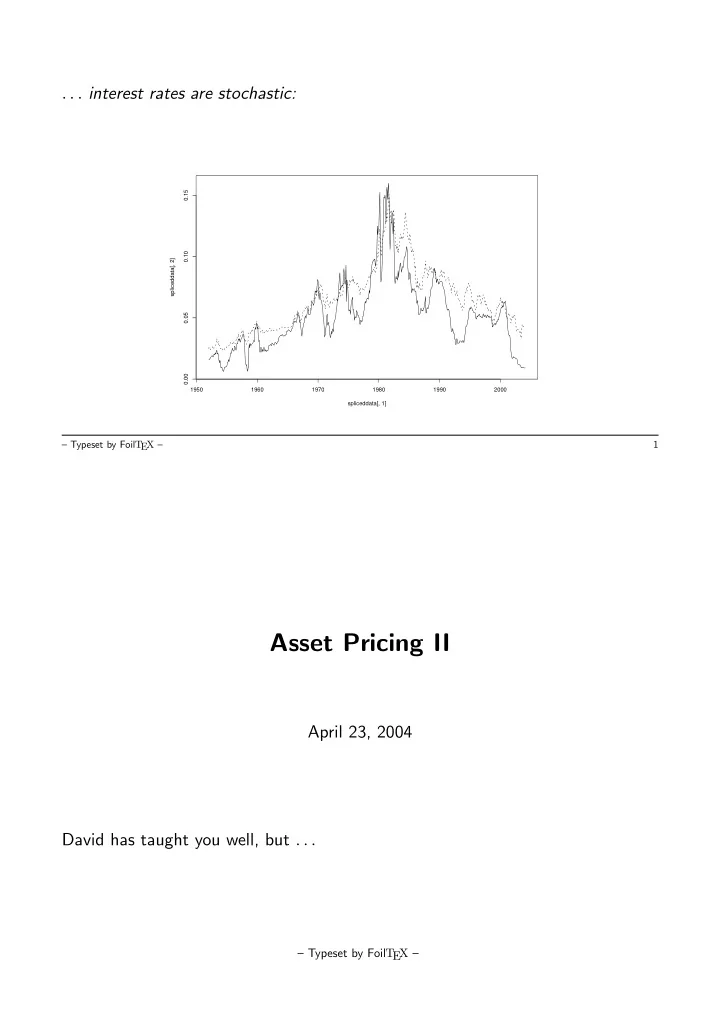
. . . interest rates are stochastic:

1950 1960 1970 1980 1990 2000 0.00 0.05 0.10 0.15 spliceddata[, 1] spliceddata[, 2]

– Typeset by FoilT EX – 1

Also in Denmark:

1995 1996 1997 1998 1999 2000 2001 2002 0.02 0.04 0.06 0.08 0.10 0.12 year zero coupon yield 1Y Amsterdam Treaty Referendum Russian Default EURO Referendum September 11 10Y 30Y Long term level

– Typeset by FoilT EX – 2

And that is what the rest of Asset Pricing II is about. Rolf: Bj¨

• rk’s Chapters 20-25 with some detours.
• Abstract nonsense, general theory, HJM-formalism. Ch. 20, 23, and 21. Today.
• Concrete models; the 1-dimensional affine short rate models. Vasicek, Cox-

Ingersoll-Ross. Loads of stuff we can calculate. And we will. And calibrate. Ch.

• 22. Today, and maybe some on May 13.
• Change of numeraire. Needed for option-pricing. Ch. 24, but I won’t do it like
• that. Definitely May 13.
• Price-formulas for options on bonds. Ch. 24. May 13, but it’s probably not

enough.

– Typeset by FoilT EX – 3

• LIBOR market models. Ch. 25. May 14.
• Multidimensional affine models. Matrix-calculations, but much the same as

1-dimensional. However, it is a considerably richer class than you’d think. And strange things can happen. May 14 in the afternoon. Literature: Hmmm, something like – Duffie & Kan, Math. Fin., 1996 – Dai & Singleton, J. Finance, 2000 – Ch. 4 in Brigo & Mercurio’s 2001-book is a nice treatment of 2-factor models. Pierre: Fancy stuff.

– Typeset by FoilT EX – 4

What determines interest rates? And what moves them around?

• Agents’ preferences for consuming now rater than later.
• Supply & demand.
• Economic growth rates.
• Expected inflation
• Fiscal policy (in the hand of politicians)
• Monetary policy (largely central banks nowadays; Greenspan)
• Labor market structure

– Typeset by FoilT EX – 5

• International effects, exchange rates.

Overload: Too much to model!

Randomness is a very large component. Let’s just accept that and build (empiri- cally plausible) stochastic models. Worked well for stocks. Complicating factor: Many assets (bonds) that are different (because they pay at different times) but not too different. That is what interest rate (or term structure or fixed income) modelling is about. (I don’t think I have to tell you that fixed income markets are huge. DK government bonds at CSX: Around 1,200 billion (1.2 × 1012) DKK. About the same in mortgage-backed bonds.)

– Typeset by FoilT EX – 6

Bj¨

• rk Chapters 20 and 23 : Abstract/general theory.

T-maturity ZCB; time-t price denoted P(t; T). As a fct of T: Smooth. As a fct

• f t: Erratic (Ito-process).

Continuously compounded ZC yield y(t, τ) is defined by P(t; t + τ) = exp(−τy(t; τ)) ⇔ y(t; τ) = −ln P(t; t + τ) τ . Note the shift from time of maturity to time to maturity. Instantaneous forward rates (mathematically convenient) f(t, T) = −∂ ln P(t; T) ∂T .

– Typeset by FoilT EX – 7

• Interpretation. Why does this make sense?

The term structure of interest rates at date t is the mapping τ → y(t; τ)

• r some translation of it (eg. into ZCB prices or forward rates). In theory this

curve is observable in practice. In practice, well . . . Short rate: r(t) = f(t; t), Bank account: β(t) = exp( t

0 r(s)ds)

Beware of interest rate quotations: Discrete vs. continuous compounding. Instan- taneous vs. “simple” rates. Yields on what? Advice: Show me the money! (& a formula, if you don’t mind)

– Typeset by FoilT EX – 8

Dynamics equations (Bj¨

• rk equations 20.1-3)

Short rate (⊤ means transposition) dr(t) = a(t)dt + b⊤(t)dW(t) (1) ZCB prices (one eqn’ for each T; note shift to prop. coefficients) dP(t; T) = m(t; T)P(t; T)dt + v⊤(t; T)P(t; T)dW(t) (2) Forward rates d f(t; T) = α(t; T)dt + σ⊤(t; T)dW(t) (3)

– Typeset by FoilT EX – 9

No financial assumptions yet. W is just BM under some measure. Coefficients are adapted (vector-valued) process, but smooth in T; subscript-T denotes T-differentiation. We have f(t; T) = −∂ ln P(t; T) ∂T ⇔ P(t; T) = exp

• −

T

t

f(t; s)ds

• and

r(t) = f(t, t). So what’s the connection?

– Typeset by FoilT EX – 10

Proposition 20.5 (Quite important result.) 1) If ZCB prices satisfy (2) then forward rates satisfy (3) with α(t; T) = v⊤

T (t; T)v(t; T) − mT(t; T)

and σ(t; T) = −vT(t; T). 2) If forward rates satisfy (3) then the short rate satisfies (1) with a(t) = fT(t, t) + α(t, t) and b(t) = σ(t; t). 3) If forward rates satisfy (3) then ZCB prices satisfy (2) with m(t; T) = r(t) + A(t; T) + 1 2S⊤(t; T)S(t; T) and v(t; T) = S(t; T),

– Typeset by FoilT EX – 11

where A(t; T) = − T

t α(t; s)ds

and S(t; T) = − T

t σ(t; s)ds.

You’ll forget terms if you aren’t careful, so let’s sketch a proof: 1): Take logs, use Ito & differentiate wrt. T 2): r(t) = f(t; t), but “the chain rule” inspires us to write dr(t) = dtf(t; T)|T =t + dTf(t; T)

• =fT (t;T )dt

|T =t and the result follows.

– Typeset by FoilT EX – 12

3): P(t; T) = exp

• −

T

t f(t; s)ds

• , so t enters in two places in an even trickier
• way. But recall the Leibniz rule:

d dx x h(t, x)dx = h(x, x) + x hx(t, x)dx. “Believe in that” for stochastic integrals too! So with Y (t; T) = − T

t f(t; s)ds

we get dY (t; T) = f(t; t)dt − T

t

d f(t; s)ds. Now plug in, interchange & use Ito on exp. Of course the only real way to prove it is to write things out in integral form, see the original HJM-article or the note on the course homepage. Takes about two hours of me writing integrals on the blackboard.

– Typeset by FoilT EX – 13

An application: The HJM drift condition

Assume that there model of forward rates is given by (3) under some measure P. Suppose further that the model is arbitrage-free. Then there exists an equivalent martingale measure Q ∼ P such that P(t; T) β(t) is a Q-martingale for all T. So dP(t; T) = r(t)P(t; T)dt + S⊤(t; T)dW Q(t).

– Typeset by FoilT EX – 14

Note the subtle application of Girsanov’s theorem: Equivalent changes of measure change drift – not volatility. But from Proposition 20.5 3) we get r(t) = r(t) + AQ(t; T) + 1 2S⊤(t; T)S(t; T) ⇒ −AQ(t; T) = 1 2S⊤(t; T)S(t; T). Differentiate both sides wrt. T and get the Heath-Jarrow-Morton drift condition αQ(t; T) = σ⊤(t; T) T

t

σ(t; s)ds.

– Typeset by FoilT EX – 15

But what about drifts under P? From Girsanov’s theorem we know that there exists a stochastic process λ such that dW Q = dW P − λ(t)dt defines a Q-BM. Important: λ doesn’t depend on T. Not important: Whether I choose to write “+” or “-”. We have dP(t; T) P(t; T) = (r(t) + AP(t; T) + 1 2S⊤(t; T)S(t; T))dt + S⊤(t; T)dW P(t) = r(t)dt + S⊤(t; T)dW Q(t) +

• AP(t; T) + 1

2S⊤(t; T)S(t; T) + S⊤(t; T)λ(t)

• must = 0

.

– Typeset by FoilT EX – 16

This means that −AP(t; T) = 1

2S⊤(t; T)S(t; T) + S⊤(t; T)λ(t). Differentiating

• wrt. T gives

αP(t; T) = σ⊤(t; T) T

t

σ(t; s) − λ(t)

• .

In sloppy matrix notation we may write λ(t) = −EP(return on ZCB) − r(t) Vol(ZCB) . If σ (forward rate volatility) is chosen positive then (typically) λ(t) will be positive. Otherwise it’s negative.

– Typeset by FoilT EX – 17

Another application (& old exam question): HJM and the Markov-property The drift condition makes the dynamics of one forward rates dependent on all

• ther forward rates ⇒ Non-markovian,

(How much has David talked about the Markov-property? If you don’t know what that is, then the statement is void.) But sometimes the models are Markovian. and here I solve the exercise There’s more literature on this where people do cunning stuff.

– Typeset by FoilT EX – 18

A third application: Musiela formulation/parametrization Change to time to maturity in forward rates: r(t, x) = f(t; t + x). “How rates are quoted” (practice) and we get an object that lives on a rectangular domain (mathematical). By the chain rule dr(t, x) = dtf(t; T)|T =t+x + dTf(t; T)|T =t+x = d f(t, t + x) + ∂ ∂x

• =F

r(t, x), and in fancy notation (see details p. 345) the drift condition gives dr(t, x) = (F(t, x) + D(t, x)) dt + σ0(t, x)

=σ(t,t+x)

dW Q(t)

– Typeset by FoilT EX – 19

The term structure can now be analyzed with tools for infinite dimensional SDEs. Very tricky stuff!

– Typeset by FoilT EX – 20

Other words you’re bound to hear

(Forward) LIBOR (rates): Definition 20.2; more in Ch. 25 Caplets & caps: (Sums of) options on LIBOR. We’ll price them later. Floating rate bonds: Easier than you’d think. Swaps: “Plain vanilla” = (floating - fixed) rate bond. Swaptions: We’ll price them later too.

– Typeset by FoilT EX – 21