Approach 5: Variance-Stabilizing Transformation For certain - - PowerPoint PPT Presentation

ST 762 Nonlinear Statistical Models for Univariate and Multivariate Response

Approach 5: Variance-Stabilizing Transformation

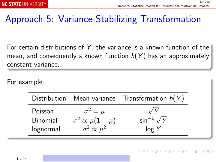
For certain distributions of Y , the variance is a known function of the mean, and consequently a known function h(Y ) has an approximately constant variance. For example: Distribution Mean-variance Transformation h(Y ) Poisson σ2 = µ √ Y Binomial σ2 ∝ µ(1 − µ) sin−1 √ Y lognormal σ2 ∝ µ2 log Y

1 / 14

ST 762 Nonlinear Statistical Models for Univariate and Multivariate Response

Empirically, transformation often was found also to make the dependence linear. So for example counted data Y , where the Poisson distribution might be relevant, might be modeled as E

• Yj
• xj
• = xT

j β,

var

• Yj
• xj
• = σ2.

Remarks We may not be so lucky! Even if we are, β is hard to interpret.

2 / 14

ST 762 Nonlinear Statistical Models for Univariate and Multivariate Response

Approach 6: Box-Cox Transformation

Let the data determine the transformation in a parametric family h(Y , λ). Box and Cox used the power family: h(Y , λ) =    Y λ − 1 λ λ = 0 log Y λ = 0. Assume linearity and normality: h (Yj, λ) ∼ N

• xT

j β, σ2

. Estimate λ, β, and σ2 by ML.

3 / 14

ST 762 Nonlinear Statistical Models for Univariate and Multivariate Response

Remarks Same issues as before. One transformation is assumed to achieve linearity, normality, and constant variance. β is hard to interpret.

4 / 14

ST 762 Nonlinear Statistical Models for Univariate and Multivariate Response

Approach 7: Transform Both Sides (TBS)

Suppose we have scientific reasons for a model f (x, β). Assume that, conditionally on xj, h (Yj, λ) = h {f (xj, β) , λ} + ej The deviations e1, e2, . . . , en satisfy the standard assumptions: constant variance σ2; independence and normality. Estimate β, λ, and σ2 by ML.

5 / 14

ST 762 Nonlinear Statistical Models for Univariate and Multivariate Response

Still requires a strong assumption. Still difficult to interpret. But: if h is smooth and invertible and σ is small relative to f (x, β), we can use a linear approximation: Yj = h−1 [h {f (xj, β) , λ} + ej, λ] ≈ f (xj, β) + 1 hy {f (xj, β) , λ} × ej where hy(y, λ) = ∂h(y, λ) ∂y .

6 / 14

ST 762 Nonlinear Statistical Models for Univariate and Multivariate Response

So to this order of approximation, E (Yj| xj) ≈ f (xj, β) and var (Yj| xj) ≈ σ2 hy {f (xj, β) , λ}2 ≈ σ2 hy {E (Yj) , λ}2. For the Box-Cox family, hy(y, λ) = y λ−1, so var (Yj| xj) ≈ σ2f (xj, β)2(1−λ) ≈ σ2E (Yj| xj)2(1−λ) .

7 / 14

ST 762 Nonlinear Statistical Models for Univariate and Multivariate Response

So: normality and constant variance on the transformed scale are (approximately) equivalent to normality and non-constant variance on the original scale, with the variance given by a certain function of the mean. Henceforth, we do not consider transformations. Instead, we model variances, and sometimes distributions, explicitly.

8 / 14

ST 762 Nonlinear Statistical Models for Univariate and Multivariate Response

Approach 8: ML for an Assumed Model

E.g. Y is a count, which we could model as Poisson-distributed, with a model for the mean: E(Y |x) = f (x, β). This implies a model for the variance, var(Y |x) = E(Y |x) = f (x, β) but we do not need it in likelihood-based inference.

9 / 14

ST 762 Nonlinear Statistical Models for Univariate and Multivariate Response

Approach 9: Generalized Least Squares (GLS)

Assume E(Y |x) = f (x, β), var(Y |x) = σ2g(β, θ, x)2. Here: β is, as before, the vector of parameters in the mean function; θ is a possible additional parameter in the structure of the variance function; σ2 is a possible over-dispersion parameter.

10 / 14

ST 762 Nonlinear Statistical Models for Univariate and Multivariate Response

Ad hoc estimation scheme:

i

Get initial estimate of β using OLS;

ii

Get initial estimate of θ, if needed, and construct initial estimated weights ˆ wj = 1 g

• ˆ

βOLS, ˆ θ, x 2

iii Re-estimate β using WLS, treating ˆ

wj as fixed: solve the estimating equation

n

• j=1

ˆ wj {Yj − f (xj, β)} fβ (xj, β) = 0.

11 / 14

ST 762 Nonlinear Statistical Models for Univariate and Multivariate Response

Remarks In step iii, equivalently, ˆ βWLS minimizes S ˆ

w(β) = n

• j=1

ˆ wj {Yj − f (xj, β)}2 . As noted before, this is a computational alternative to solving the estimating equation, but is not generally preferred. The estimating-equation approach may be extended to cases where no such objective function exists. Could repeat step ii with ˆ βWLS instead of ˆ βOLS, then repeat step iii. We could also iterate, perhaps to convergence.

12 / 14

ST 762 Nonlinear Statistical Models for Univariate and Multivariate Response

Approach 10: ML

Same moment structure as in Approach 9: E(Y |x) = f (x, β), var(Y |x) = σ2g(β, θ, x)2. Add an assumption about the distribution of Y |x: Y = f (x, β) + σg(β, θ, x)Z where Z has mean 0 and variance 1, such as N(0, 1), and use likelihood methods. When g(·) involves β, the ML estimating equation for β is not the same as in GLS.

13 / 14

ST 762 Nonlinear Statistical Models for Univariate and Multivariate Response

Comments on Approaches 5–10

Approaches 5–7 require (lucky) transformation, and the parameters can be hard for interpretation. Approaches 8–10 are the most interesting. Depending on the form of the functions f (·) and g(·), these approaches will sometimes yield the same estimating equations.

14 / 14