Applied Machine Learning CIML Chap 4 (A Geometric Approach) - PowerPoint PPT Presentation

Applied Machine Learning CIML Chap 4 (A Geometric Approach) “ Equations are just the boring part of mathematics. I attempt to see things in terms of geometry. ” ― Stephen Hawking Week 4: Linear Classification: Perceptron Professor Liang Huang some slides from Alex Smola (CMU/Amazon)

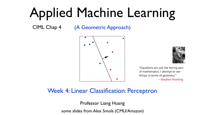
Roadmap for Unit 2 (Weeks 4-5) • Week 4: Linear Classifier and Perceptron • Part I: Brief History of the Perceptron • Part II: Linear Classifier and Geometry (testing time) • Part III: Perceptron Learning Algorithm (training time) • Part IV: Convergence Theorem and Geometric Proof • Part V: Limitations of Linear Classifiers, Non-Linearity, and Feature Maps • Week 5: Extensions of Perceptron and Practical Issues • Part I: My Perceptron Demo in Python • Part II: Voted and Averaged Perceptrons • Part III: MIRA and Aggressive MIRA • Part IV: Practical Issues • Part V: Perceptron vs. Logistic Regression (hard vs. soft); Gradient Descent 2

Part I • Brief History of the Perceptron 3

Perceptron (1959-now) Frank Rosenblatt

deep learning 
 ~1986; 2006-now multilayer perceptron logistic regression 
 perceptron 
 SVM 
 1958 
 1964;1995 1958 kernels 
 1964 cond. random fields 
 structured SVM 
 structured perceptron 
 2001 
 2003 
 2002 5

Neurons • Soma (CPU) 
 Cell body - combines signals • Dendrite (input bus) 
 Combines the inputs from 
 several other nerve cells • Synapse (interface) 
 Interface and parameter store between neurons • Axon (output cable) 
 May be up to 1m long and will transport the activation signal to neurons at different locations 6

Frank Rosenblatt’s Perceptron 7

Multilayer Perceptron (Neural Net) 8

Brief History of Perceptron batch 1997 +soft-margin Cortes/Vapnik SVM +kernels online approx. 
 subgradient descent max margin +max margin 2007--2010 minibatch Singer group Pegasos minibatch online 2003 2006 Crammer/Singer Singer group conservative updates MIRA aggressive 1958 1962 1969* 1999 DEAD Rosenblatt Novikoff Minsky/Papert Freund/Schapire invention proof book killed it voted/avg: revived inseparable case 2002 2005* Collins McDonald/Crammer/Pereira structured structured MIRA *mentioned in lectures but optional 
 (others papers all covered in detail) AT&T Research ex-AT&T and students 9

Part II • Linear Classifier and Geometry (testing time) • decision boundary and normal vector w • not separable through the origin: add bias b • geometric review of linear algebra • augmented space (no explicit bias; implicit as w 0 = b ) Test Time Input x Prediction σ ( w · x ) Linear Classifier Model w Training Time Input x Model w Perceptron Learner Output y 10

Linear Classifier and Geometry linear classifiers: perceptron, logistic regression, (linear) SVMs, etc. x n x 1 x 2 x 3 . . . x 2 k x k cos θ = w · x w n w 1 k w k weights x output f ( x ) = σ ( w · x ) σ θ O negative x 1 w w · x < 0 positive weight vector w is a “prototype” of positive examples w · x > 0 it’s also the normal vector of the decision boundary meaning of w · x : agreement with positive direction 
 separating hyperplane 
 test : input: x , w ; output:1 if w · x >0 else -1 (decision boundary) training : input: ( x , y ) pairs; output: w 11 w · x = 0

What if not separable through origin? solution: add bias b x n x 1 x 2 x 3 . . . x 2 = w · x k x k cos θ w n w 1 k w k weights x output f ( x ) = σ ( w · x + b ) θ O negative x 1 w w · x + b < 0 positive w · x + b > 0 w · x + b = 0 | b | k w k 12

Geometric Review of Linear Algebra line in 2D ( n -1)-dim hyperplane in n -dim x 2 x 2 w · x + b = 0 w 1 x 1 + w 2 x 2 + b = 0 x ∗ ( x ∗ 1 , x ∗ 2 ) | b | k ( w 1 , w 2 ) k ( w 1 , w 2 ) O O x 1 x 1 required: algebraic and geometric meanings of dot product x 3 | w 1 x ∗ 2 + b | | w · x + b | 1 + w 2 x ∗ = | ( w 1 , w 2 ) · ( x 1 , x 2 ) + b | p k ( w 1 , w 2 ) k w 2 1 + w 2 k w k 2 point-to-line distance point-to-hyperplane distance 13 LA-geom

Augmented Space: dimensionality+1 explicit bias x n x 1 x 2 x 3 . . . f ( x ) = σ ( w · x + b ) w n w 1 can’t separate in 1D 
 weights from the origin O output x 0 = 1 augmented space x 3 x n x 1 x 2 . . . w 0 = b f ( x ) = σ (( b ; w ) · (1; x )) w n w 1 weights 1 can separate in 2D 
 from the origin O output 14

Augmented Space: dimensionality+1 explicit bias x n x 1 x 2 x 3 . . . f ( x ) = σ ( w · x + b ) w n w 1 can’t separate in 2D 
 weights from the origin output x 0 = 1 augmented space x 3 x n x 1 x 2 . . . w 0 = b f ( x ) = σ (( b ; w ) · (1; x )) w n w 1 weights can separate in 3D 
 from the origin output 15

Part III • The Perceptron Learning Algorithm (training time) • the version without bias (augmented space) • side note on mathematical notations • mini-demo Test Time Input x Prediction σ ( w · x ) Linear Classifier Model w Training Time Input x Model w Perceptron Learner Output y 16

Perceptron Ham Spam 17

The Perceptron Algorithm input: training data D x output: weights w initialize w ← 0 while not converged w 0 aa for ( x , y ) ∈ D aaaa if y ( w · x ) ≤ 0 aaaaaa w ← w + y x w • the simplest machine learning algorithm • keep cycling through the training data • update w if there is a mistake on example ( x , y ) • until all examples are classified correctly 18

Side Note on Mathematical Notations • I’ll try my best to be consistent in notations • e.g., bold-face for vectors, italic for scalars, etc. • avoid unnecessary superscripts and subscripts by using a “Pythonic” rather than a “C” notational style • most textbooks have consistent but bad notations initialize w = 0 and b = 0 initialize w ← 0 repeat while not converged if y i [ h w, x i i + b ]  0 then aa for ( x , y ) ∈ D w w + y i x i and b b + y i aaaa if y ( w · x ) ≤ 0 end if aaaaaa w ← w + y x until all classified correctly good notations: 
 bad notations: 
 consistent, Pythonic style inconsistent, unnecessary i and b 19

Demo ← while not converged aa for ( x , y ) ∈ D aaaa if y ( w · x ) ≤ 0 aaaaaa w ← w + y x x w 0 w (bias=0) 20

Demo ← while not converged aa for ( x , y ) ∈ D aaaa if y ( w · x ) ≤ 0 aaaaaa w ← w + y x x w 21

Demo ← while not converged aa for ( x , y ) ∈ D aaaa if y ( w · x ) ≤ 0 aaaaaa w ← w + y x x w 0 w 22

Demo ← while not converged aa for ( x , y ) ∈ D aaaa if y ( w · x ) ≤ 0 aaaaaa w ← w + y x w 23

24

Part IV • Linear Separation, Convergence Theorem and Proof • formal definition of linear separation • perceptron convergence theorem • geometric proof • what variables affect convergence bound? 25

Linear Separation; Convergence Theorem • dataset D is said to be “linearly separable” if there exists some unit oracle vector u : ∣∣ u || = 1 which correctly classifies every example ( x , y ) with a margin at least ẟ : 
 y ( u · x ) ≥ δ for all ( x , y ) ∈ D • then the perceptron must converge to a linear separator after at most R 2 / ẟ 2 mistakes (updates) where ( x ,y ) ∈ D k x k R = max • convergence rate R 2 / ẟ 2 δ δ x ⊕ ⊕ • dimensionality independent u · x ≥ δ R • dataset size independent u : k u k = 1 • order independent (but order matters in output) • scales with ‘difficulty’ of problem

Geometric Proof, part 1 • part 1: progress (alignment) on oracle projection assume w (0) = 0 , and w ( i ) is the weight before the i th update (on ( x , y )) w ( i +1) = w ( i ) + y x u · w ( i +1) = u · w ( i ) + y ( u · x ) u · w ( i +1) ≥ u · w ( i ) + δ y ( u · x ) ≥ δ for all ( x , y ) ∈ D u · w ( i +1) ≥ i δ δ δ x ⊕ ⊕ projection on u increases! u · x ≥ δ (more agreement w/ oracle direction) u : k u k = 1 � w ( i +1) � � � � w ( i +1) � � � u · w ( i +1) � i δ w ( i +1) w � = k u k � � � � ( i ) u · w ( i ) 27 u · w ( i +1)

Geometric Proof, part 2 • part 2: upperbound of the norm of the weight vector w ( i +1) = w ( i ) + y x iR √ i δ 2 2 � w ( i +1) � � � w ( i ) + y x � � = � � � � � � 2 + k x k 2 + 2 y ( w ( i ) · x ) � w ( i ) � � = � � � mistake on x 2 � w ( i ) � � + R 2  x � � � ⊕ ⊕ ( x ,y ) ∈ D k x k R = max  iR 2 R Combine with part 1: w ( i +1) w � w ( i +1) � � � w ( i +1) � � � � u · w ( i +1) � i δ ( i ) � = k u k � � � � � θ ≥ 90 cos θ ≤ 0 i ≤ R 2 / δ 2 w ( i ) · x ≤ 0 28

Convergence Bound R 2 / δ 2 • is independent of: • dimensionality • number of examples • order of examples • constant learning rate narrow margin: 
 wide margin: 
 hard to separate easy to separate • and is dependent of: • separation difficulty (margin ẟ ) • feature scale (radius R ) • initial weight w (0) • changes how fast it converges, but not whether it’ll converge 29

Part V • Limitations of Linear Classifiers and Feature Maps • XOR: not linearly separable • perceptron cycling theorem • solving XOR: non-linear feature map • “preview demo”: SVM with non-linear kernel • redefining “linear” separation under feature map 30