Announcements U nit 4: I nference for numerical variables L ecture 1: - - PowerPoint PPT Presentation

Unit 4: Inference for numerical variables Lecture 1: Two samples - paired and independent Statistics 101

Mine C ¸ etinkaya-Rundel October 10, 2013

Announcements

Announcements

Midterm evaluation for course.

Statistics 101 (Mine C ¸ etinkaya-Rundel) U4 - L1: Paired and independent October 10, 2013 2 / 26 Comparing means of two groups

Comparing means of two groups

When comparing the means of two groups, we must first think about whether the data are independent or dependent across the groups: dependent (paired) groups (e.g. pre/post weights of subjects in a weight loss study) independent groups (e.g. grades of students across two sections)

Statistics 101 (Mine C ¸ etinkaya-Rundel) U4 - L1: Paired and independent October 10, 2013 3 / 26 Paired data Paired observations

200 observations were randomly sampled from the High School and Beyond survey. The same students took a reading and writing test and their scores are shown below. At a first glance, does there appear to be a difference between the average reading and writing test score?

scores 20 40 60 80 100 read write

Statistics 101 (Mine C ¸ etinkaya-Rundel) U4 - L1: Paired and independent October 10, 2013 4 / 26

Paired data Paired observations

Clicker question The same students took a reading and writing test and their scores are shown below. Are the reading and writing scores of a given student independent of each other?

id read write 1 70 57 52 2 86 44 33 3 141 63 44 4 172 47 52

. . . . . . . . . . . .

200 137 63 65

(a) Yes (b) No

Statistics 101 (Mine C ¸ etinkaya-Rundel) U4 - L1: Paired and independent October 10, 2013 5 / 26 Paired data Paired observations

Analyzing paired data

When two sets of observations have this special correspondence (not independent), they are said to be paired. To analyze paired data, it is often useful to look at the difference in outcomes of each pair of observations. diff = read − write It is important that we always subtract using a consistent order.

id read write diff 1 70 57 52 5 2 86 44 33 11 3 141 63 44 19 4 172 47 52

• 5

. . . . . . . . . . . . . . .

200 137 63 65

• 2

differences Frequency −20 −10 10 20 10 20 30 40

Statistics 101 (Mine C ¸ etinkaya-Rundel) U4 - L1: Paired and independent October 10, 2013 6 / 26 Paired data Paired observations

Parameter and point estimate

Parameter of interest: Average difference between the reading and writing scores of all high school students.

µdiff

Point estimate: Average difference between the reading and writing scores of sampled high school students.

¯

xdiff

Statistics 101 (Mine C ¸ etinkaya-Rundel) U4 - L1: Paired and independent October 10, 2013 7 / 26 Paired data Inference for paired data

Setting the hypotheses

If in fact there was no difference between the scores on the reading and writing exams, what would you expect the average difference to be? What are the hypotheses for testing if there is a difference between the average reading and writing scores? H0: There is no difference between the average reading and writing score.

µdiff = 0

HA: There is a difference between the average reading and writing score.

µdiff 0

Statistics 101 (Mine C ¸ etinkaya-Rundel) U4 - L1: Paired and independent October 10, 2013 8 / 26

Paired data Inference for paired data

Nothing new here

The analysis is no different than what we have done before. We have data from one sample: differences. We are testing to see if the average difference is different than 0.

Statistics 101 (Mine C ¸ etinkaya-Rundel) U4 - L1: Paired and independent October 10, 2013 9 / 26 Paired data Inference for paired data

Checking assumptions & conditions

Clicker question Which of the following is true? (a) Since students are sampled randomly and are less than 10% of all high school students, we can assume that the difference between the reading and writing scores of one student in the sample is independent of another. (b) The distribution of differences is bimodal, therefore we cannot continue with the hypothesis test. (c) In order for differences to be random we should have sampled with replacement. (d) Since students are sampled randomly and are less than 10% all students, we can assume that the sampling distribution of the average difference will be nearly normal.

Statistics 101 (Mine C ¸ etinkaya-Rundel) U4 - L1: Paired and independent October 10, 2013 10 / 26 Paired data Inference for paired data

Application exercise:

Work in teams: The observed average difference between the two scores is -0.545 points and the standard deviation of the difference is 8.887 points. Which of the below is the closest p-value for evaluating a difference between the average scores on the two exams? In addition, write out the interpretation

• f the p-value in context of the data and the research question.

(a) 20% (b) 40% (c) 5% (d) 48% (e) 95%

Statistics 101 (Mine C ¸ etinkaya-Rundel) U4 - L1: Paired and independent October 10, 2013 11 / 26 Paired data Inference for paired data

HT ↔ CI

Clicker question Suppose we were to construct a 95% confidence interval for the av- erage difference between the reading and writing scores. Would you expect this interval to include 0? (a) yes (b) no (c) cannot tell from the information given

Statistics 101 (Mine C ¸ etinkaya-Rundel) U4 - L1: Paired and independent October 10, 2013 12 / 26

Difference of two means Confidence intervals for differences of means

The General Social Survey (GSS) conducted by the Census Bureau contains a standard ‘core’ of demographic, behavioral, and attitudinal questions, plus topics of special interest. Many of the core questions have remained unchanged since 1972 to facilitate time-trend studies as well as replication of earlier findings. Below is an excerpt from the 2010 data set. The variables are number of hours worked per week and highest educational attainment. degree hrs1 1 BACHELOR 55 2 BACHELOR 45 3 JUNIOR COLLEGE 45

. . .

1172 HIGH SCHOOL 40

Statistics 101 (Mine C ¸ etinkaya-Rundel) U4 - L1: Paired and independent October 10, 2013 13 / 26 Difference of two means Confidence intervals for differences of means

Exploratory analysis

What can you say about the relationship between educational attain- ment and hours worked per week?

• Less than HS

HS Jr Coll Bachelor's Graduate 20 40 60 80

Statistics 101 (Mine C ¸ etinkaya-Rundel) U4 - L1: Paired and independent October 10, 2013 14 / 26 Difference of two means Confidence intervals for differences of means

Collapsing levels into two

Say we are only interested the difference between the number of hours worked per week by college and non-college graduates. Then we combine the levels of education into two: hs or lower ← less than high school or high school coll or higher ← junior college, bachelor’s, and graduate

Statistics 101 (Mine C ¸ etinkaya-Rundel) U4 - L1: Paired and independent October 10, 2013 15 / 26 Difference of two means Confidence intervals for differences of means

Using R: Construct new variable

gss = read.csv("http://stat.duke.edu/courses/Summer13/ sta104.01-1/resources/data/gss.csv") # create a new empty variable gss$edu = NA # if statements to determine levels of new variable gss$edu[gss$degree == "LESS THAN HIGH SCHOOL" | gss$degree == "HIGH SCHOOL"] = "hs or lower" gss$edu[gss$degree == "JUNIOR COLLEGE" | gss$degree == "BACHELOR" | gss$degree == "GRADUATE"] = "coll or higher" # make sure new variable is categorical gss$edu = as.factor(gss$edu)

Statistics 101 (Mine C ¸ etinkaya-Rundel) U4 - L1: Paired and independent October 10, 2013 16 / 26

Difference of two means Confidence intervals for differences of means

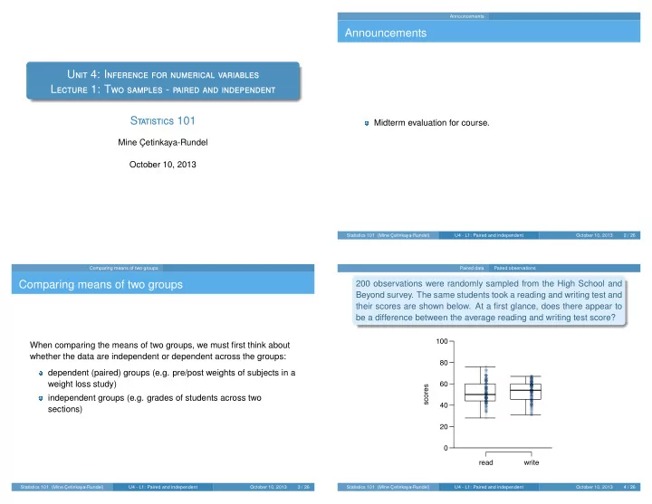
Exploratory analysis - another look

¯ x s n coll or higher 41.8 15.14 505 hs or lower 39.4 15.12 667

coll or higher

20 40 60 80 100

hs or lower

hours worked per week 20 40 60 80 150

by(gss$hrs1, gss$edu, summary) by(gss$hrs1, gss$edu, sd) by(gss$hrs1, gss$edu, length)

Statistics 101 (Mine C ¸ etinkaya-Rundel) U4 - L1: Paired and independent October 10, 2013 17 / 26 Difference of two means Confidence intervals for differences of means

Parameter and point estimate

We want to construct a 95% confidence interval for the average dif- ference between the number of hours worked per week by Americans with a college degree and those with a high school degree or lower. What are the parameter of interest and the point estimate? Parameter of interest: Average difference between the number of hours worked per week by all Americans with a college degree and those with a high school degree or lower.

µcoll − µhs

Point estimate: Average difference between the number of hours worked per week by sampled Americans with a college degree and those with a high school degree or lower.

¯

xcoll − ¯ xhs

Statistics 101 (Mine C ¸ etinkaya-Rundel) U4 - L1: Paired and independent October 10, 2013 18 / 26 Difference of two means Confidence intervals for differences of means

Checking assumptions & conditions

1

Independence:

Within groups:

both samples are random 505 < 10% of all college graduates and 667 < 10% of all students with a high school degree or lower,

We can assume that the number of hours worked per week by

• ne college graduate in the sample is independent of another,

and the number of hours worked per week by someone with a HS degree or lower in the sample is independent of another as well. Between groups: ← new! Since the sample is random, we have no reason to believe that the college graduates in the sample would not be independent of those with a HS degree or lower.

2

Sample size / skew: Both distributions look reasonably symmetric, and the sample sizes are at least 30, therefore we can assume that the sampling distribution of number of hours worked per week by college graduates and those with HS degree or lower are nearly normal. Hence the sampling distribution of the average difference will be nearly normal as well.

Statistics 101 (Mine C ¸ etinkaya-Rundel) U4 - L1: Paired and independent October 10, 2013 19 / 26 Difference of two means Confidence intervals for differences of means

Confidence interval for difference between two means

All confidence intervals have the same form: point estimate ± ME And all ME = critical value × SE of point estimate In this case the point estimate is ¯ x1 − ¯ x2 Since the sample sizes are large enough, the critical value is z⋆ So the only new concept is the standard error of the difference between two means... Standard error of the difference between two sample means SE(¯

x1−¯ x2) =

• s2

1

n1

+

s2

2

n2

Statistics 101 (Mine C ¸ etinkaya-Rundel) U4 - L1: Paired and independent October 10, 2013 20 / 26

Difference of two means Confidence intervals for differences of means

Let’s put things in context

Calculate the standard error of the average difference between the number of hours worked per week by college graduates and those with a HS degree or lower.

¯

x s n coll or higher 41.8 15.14 505 hs or lower 39.4 15.12 667 SE(¯

xcoll−¯ xhs)

=

• s2

coll

ncoll

+

s2

hs

nhs

=

• 15.142

505

+ 15.122

667

=

0.89

Statistics 101 (Mine C ¸ etinkaya-Rundel) U4 - L1: Paired and independent October 10, 2013 21 / 26 Difference of two means Confidence intervals for differences of means

Confidence interval for the difference (cont.)

Estimate (using a 95% confidence interval) the average difference be- tween the number of hours worked per week by Americans with a col- lege degree and those with a high school degree or lower.

¯

xcoll = 41.8

¯

xhs = 39.4 SE(¯

xcoll−¯ xhs) = 0.89

(¯

xcoll − ¯ xhs) ± z⋆ × SE(¯

xcoll−¯ xhs)

= (41.8 − 39.4) ± 1.96 × 0.89 =

2.4 ± 1.74

= (0.66, 4.14)

Statistics 101 (Mine C ¸ etinkaya-Rundel) U4 - L1: Paired and independent October 10, 2013 22 / 26 Difference of two means Confidence intervals for differences of means

Interpretation of a confidence interval for the difference

Clicker question Which of the following is the best interpretation of the confidence inter- val we just calculated? We are 95% confident that (a) the difference between the average number of hours worked per week by college grads and those with a HS degree or lower is between 0.66 and 4.14 hours. (b) college grads work on average of 0.66 to 4.14 hours more per week than those with a HS degree or lower. (c) college grads work on average 0.66 hours less to 4.14 hours more per week than those with a HS degree or lower. (d) college grads work on average 0.66 to 4.14 hours less per week than those with a HS degree or lower.

Statistics 101 (Mine C ¸ etinkaya-Rundel) U4 - L1: Paired and independent October 10, 2013 23 / 26 Difference of two means Confidence intervals for differences of means

Reality check

Do these results sound reasonable? Why or why not?

Statistics 101 (Mine C ¸ etinkaya-Rundel) U4 - L1: Paired and independent October 10, 2013 24 / 26

Difference of two means Hypothesis tests for differences of means

Setting the hypotheses

What are the hypotheses for testing if there is a difference between the average number of hours worked per week by college graduates and those with a HS degree or lower? H0: µcoll = µhs

There is no difference in the average number of hours worked per week by college graduates and those with a HS degree or lower. Any

• bserved difference between the sample means is due to natural

sampling variation (chance).

HA: µcoll µhs

There is a difference in the average number of hours worked per week by college graduates and those with a HS degree or lower.

Statistics 101 (Mine C ¸ etinkaya-Rundel) U4 - L1: Paired and independent October 10, 2013 25 / 26 Difference of two means Hypothesis tests for differences of means

Application exercise: Work in teams: Calculate the test-statistic and the p-value, and write

• ut your conclusion

H0: µcoll = µhs → µcoll − µhs = 0 HA: µcoll µhs → µcoll − µhs 0

¯

xcoll − ¯ xhs = 2.4, SE(¯ xcoll − ¯ xhs) = 0.89

Statistics 101 (Mine C ¸ etinkaya-Rundel) U4 - L1: Paired and independent October 10, 2013 26 / 26