Announcements Wednesday, October 18 The second midterm is on this - PowerPoint PPT Presentation

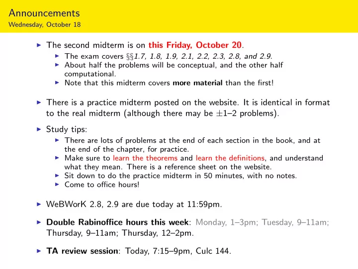
Announcements Wednesday, October 18 ◮ The second midterm is on this Friday, October 20 . ◮ The exam covers §§ 1.7, 1.8, 1.9, 2.1, 2.2, 2.3, 2.8, and 2.9. ◮ About half the problems will be conceptual, and the other half computational. ◮ Note that this midterm covers more material than the first! ◮ There is a practice midterm posted on the website. It is identical in format to the real midterm (although there may be ± 1–2 problems). ◮ Study tips: ◮ There are lots of problems at the end of each section in the book, and at the end of the chapter, for practice. ◮ Make sure to learn the theorems and learn the definitions, and understand what they mean. There is a reference sheet on the website. ◮ Sit down to do the practice midterm in 50 minutes, with no notes. ◮ Come to office hours! ◮ WeBWorK 2.8, 2.9 are due today at 11:59pm. ◮ Double Rabinoffice hours this week : Monday, 1–3pm; Tuesday, 9–11am; Thursday, 9–11am; Thursday, 12–2pm. ◮ TA review session : Today, 7:15–9pm, Culc 144.

Midterm 2 Review Slides

Transformations Vocabulary Definition A transformation (or function or map ) from R n to R m is a rule T that assigns to each vector x in R n a vector T ( x ) in R m . ◮ R n is called the domain of T (the inputs). ◮ R m is called the codomain of T (the outputs). ◮ For x in R n , the vector T ( x ) in R m is the image of x under T . Notation: x �→ T ( x ). ◮ The set of all images { T ( x ) | x in R n } is the range of T . Notation: T : R n − T is a transformation from R n to R m . → R m means It may help to think of T as a “machine” that takes x T as an input, and gives you x T ( x ) as the output. T ( x ) range T R n R m domain codomain

Matrix Transformations If A is an m × n matrix, then T : R n → R m defined by T ( x ) = Ax is a matrix transformation . These are the kinds of transformations we can use linear algebra to study, because they come from matrices . � 1 � 2 3 Example: A = 4 5 6   x  = T y  z (Note we’ve written a formula for T that doesn’t a priori have anything to do with matrices.)

Questions about Transformations Here are some natural questions that one can ask about a general transformation (not just on the midterm, but in the real world too): Question: What kind of vectors can you input into T ? What kind of vectors do you get out? In other words, what are the domain and codomain? Answer for T ( x ) = Ax : Inputs are in R n , where n is the number of columns of T . Outputs are in R m , where m is the number of rows of A . (Cf. previous slide.) Question: For which b does T ( x ) = b have a solution? In other words, what is the range of T ? Answer for T ( x ) = Ax : The range is Col A , the span of the columns: T ( x ) = Ax is a linear combination of the columns of A . Question: Is T one-to-one, onto, and/or invertible? Answer for T ( x ) = Ax : on the next slides

One-to-one and onto Definition A transformation T : R n → R m is: ◮ one-to-one if T ( x ) = b has at most one solution for every b in R m ◮ onto if T ( x ) = b has at least one solution for every b in R m Picture: [interactive] This is neither one-to-one nor onto. ◮ Can you find two different solutions to T ( x ) = 0? ◮ Can you find a b such that T ( x ) = b has no solution? Picture: [interactive] This is onto but not one-to-one. ◮ Can you find two different solutions to T ( x ) = 0? Picture: [interactive] This is one-to-one and onto.

One-to-one and Onto Matrix Transformations Theorem Let T : R n → R m be a matrix transformation with matrix A . Then the following are equivalent: ◮ T is one-to-one ◮ T ( x ) = b has one or zero solutions for every b in R m ◮ Ax = b has a unique solution or is inconsistent for every b in R m ◮ Ax = 0 has a unique solution ◮ The columns of A are linearly independent ◮ A has a pivot in column . Theorem Let T : R n → R m be a matrix transformation with matrix A . Then the following are equivalent: ◮ T is onto ◮ T ( x ) = b has a solution for every b in R m ◮ Ax = b is consistent for every b in R m ◮ The columns of A span R m ◮ A has a pivot in every row

Linear Transformations Question: How do you know if a transformation is a matrix transformation or not? Definition A transformation T : R n → R m is linear if it satisfies the the equations T ( u + v ) = T ( u ) + T ( v ) and T ( cv ) = cT ( v ) . for all vectors u , v in R n and all scalars c . ( = ⇒ T (0) = 0) Theorem Let T : R n → R m be a linear transformation. Then T is a matrix transformation with matrix   | | |  . A = T ( e 1 ) T ( e 2 ) · · · T ( e n )  | | | So a linear transformation is a matrix transformation, where you haven’t computed the matrix yet. Important You compute the columns of the matrix for T by plugging in e 1 , e 2 , . . . , e n .

Examples Example: T : R → R defined by T ( x ) = x + 1. This is not linear: T (0) = 1 � = 0. Example: T : R 2 → R 2 defined by rotation by θ degrees. Is T linear? Check: The pictures show T ( u )+ T ( v ) = T ( u + v ) and T ( cu ) = cT ( u ), so T is linear.

Examples Continued Example: T : R 2 → R 2 defined by rotation by θ degrees. What is the standard matrix?

✧ Examples Continued Example: T : R 3 → R 2 defined by   x � 2 x + 3 y − z �  = T y .  y + z z Is T linear? Check T ( u + v ) = T ( u ) + T ( v ): Note we’re treating u and v as unknown vectors: this has to work for all vectors u and v !

✧ Examples Continued Example: T : R 3 → R 2 defined by   x � 2 x + 3 y − z �  = T y .  y + z z Is T linear? Check T ( cu ) = cT ( u ): Conclusion: T is linear.

Examples Continued Example: T : R 3 → R 2 defined by   x � 2 x + 3 y − z �  = T y .  y + z z We know it is linear, so it is a matrix transformation. What is its standard matrix A ?

Subspaces Definition A subspace of R n is a subset V of R n satisfying: 1. The zero vector is in V . “not empty” 2. If u and v are in V , then u + v is also in V . “closed under addition” 3. If u is in V and c is in R , then cu is in V . “closed under × scalars” A subspace is a span, and a span is a subspace. Important examples of subspaces: ◮ The span of any set of vectors. ◮ The column space of a matrix. ◮ The null space of a matrix. ◮ The solution set of a system of homogeneous equations. ◮ All of R n and the zero subspace { 0 } .

Subspaces What is the point? The point of a subspace is to talk about a span without figuring out which vectors it’s the span of.   2 7 − 4 3 Example: A = 0 0 12 1 V = Nul A   0 0 0 − 78 There are 3 pivots, so rank A = 3. By the rank theorem, dim Nul A = 1. We know the null space is a line, but we never had to compute a spanning vector!