Announcements A1 due this Friday Motion and optical flow Tues Feb - PDF document

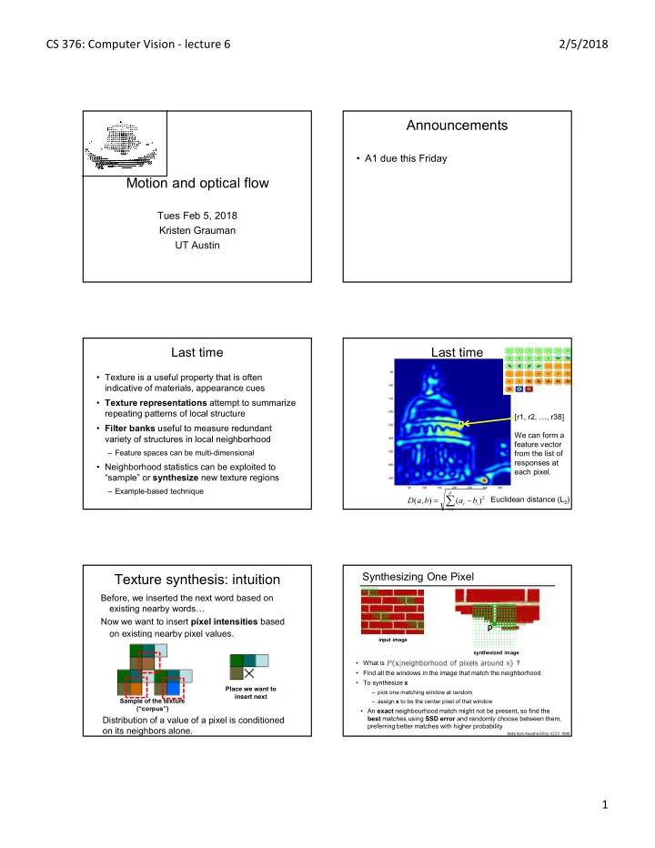
CS 376: Computer Vision - lecture 6 2/5/2018 Announcements • A1 due this Friday Motion and optical flow Tues Feb 5, 2018 Kristen Grauman UT Austin Last time Last time • Texture is a useful property that is often indicative of materials, appearance cues • Texture representations attempt to summarize repeating patterns of local structure [r1, r2, …, r38] • Filter banks useful to measure redundant We can form a variety of structures in local neighborhood feature vector – Feature spaces can be multi-dimensional from the list of responses at • Neighborhood statistics can be exploited to each pixel. “sample” or synthesize new texture regions – Example-based technique d  D ( a , b )  ( a  b ) 2 Euclidean distance (L 2 ) i i  i 1 Texture synthesis: intuition Synthesizing One Pixel Before, we inserted the next word based on existing nearby words… Now we want to insert pixel intensities based p on existing nearby pixel values . input image synthesized image • What is ? • Find all the windows in the image that match the neighborhood • To synthesize x Place we want to – pick one matching window at random insert next Sample of the texture – assign x to be the center pixel of that window (“corpus”) • An exact neighbourhood match might not be present, so find the Distribution of a value of a pixel is conditioned best matches using SSD error and randomly choose between them, preferring better matches with higher probability on its neighbors alone. Slide from Alyosha Efros, ICCV 1999 1

CS 376: Computer Vision - lecture 6 2/5/2018 How to evaluate texture Neighborhood Window generation? input Slide from Alyosha Efros, ICCV 1999 Image Quilting [Efros & Freeman 2001] • The Efros & Leung algorithm non-parametric sampling – Simple p – Surprisingly good results B – Synthesis is easier than analysis! Input image Synthesizing a block – …but very slow • Observation: neighbor pixels are highly correlated Idea: unit of synthesis = block • Exactly the same but now we want P( B |N( B )) • Much faster: synthesize all pixels in a block at once Slide from Alyosha Efros, ICCV 1999 Minimal error boundary block Input texture overlapping blocks vertical boundary B1 B2 B1 B2 B1 B2 Random placement Neighboring blocks Minimal error constrained by overlap boundary cut of blocks 2 _ = overlap error min. error boundary Slide from Alyosha Efros 2

CS 376: Computer Vision - lecture 6 2/5/2018 Texture Transfer parmesan • Take the texture from one object and “paint” it onto + = another object – This requires separating texture and shape – That’s HARD, but we can cheat – Assume we can capture shape rice by boundary and rough + = shading • Then, just add another constraint when sampling: similarity to underlying image at that spot Slide credit: Freeman & Efros (Manual) texture synthesis in the media + = Video textures Arno Schodl, Richard Szeliski, David H. Salesin, and Irfan Essa. Video textures. Proceedings of SIGGRAPH 2000 , pages 489-498, July 2000. 3

CS 376: Computer Vision - lecture 6 2/5/2018 Style transfer Today • Optical flow: estimating motion in video • Background subtraction https://www.youtube.com/watch?v=Khuj4ASldmU Video Uses of motion • A video is a sequence of frames captured • Estimating 3D structure over time • Segmenting objects based on motion cues • Now our image data is a function of space • Learning dynamical models (x, y) and time (t) • Recognizing events and activities • Improving video quality (motion stabilization) Motion field Motion parallax • The motion field is the projection of the 3D http://psych.hanover.edu/KRANTZ/MotionParall scene motion into the image ax/MotionParallax.html 4

CS 376: Computer Vision - lecture 6 2/5/2018 Motion field + camera motion Motion field + camera motion Length of flow vectors inversely proportional to Zoom out Zoom in Pan right to left depth Z of 3d point points closer to the camera move more quickly across the image plane Figure from Michael Black, Ph.D. Thesis Motion estimation techniques Optical flow • Direct methods • Definition: optical flow is the apparent motion of brightness patterns in the image • Directly recover image motion at each pixel from spatio-temporal image brightness variations • Ideally, optical flow would be the same as the • Dense motion fields, but sensitive to appearance variations motion field • Suitable for video and when image motion is small • Have to be careful: apparent motion can be • Feature-based methods caused by lighting changes without any • Extract visual features (corners, textured areas) and track them actual motion over multiple frames • Sparse motion fields, but more robust tracking • Suitable when image motion is large (10s of pixels) Problem definition: optical flow Apparent motion != motion field How to estimate pixel motion from image H to image I? • Solve pixel correspondence problem – given a pixel in H, look for nearby pixels of the same color in I Key assumptions • color constancy: a point in H looks the same in I – For grayscale images, this is brightness constancy • small motion : points do not move very far Figure from Horn book This is called the optical flow problem 5

CS 376: Computer Vision - lecture 6 2/5/2018 Color/brightness constancy Optical flow constraints Let’s look at these constraints more closely • brightness constancy: Q: what’s the equation?    H ( x , y ) I ( x u , y v ) • small motion: Figure by Michael Black Optical flow equation Optical flow equation Combining these two equations Q: how many unknowns and equations per pixel? The aperture problem The aperture problem    I ( u ' , v ' ) 0 Actual motion Perceived motion 6

CS 376: Computer Vision - lecture 6 2/5/2018 The barber pole illusion Solving the aperture problem • How to get more equations for a pixel? • Spatial coherence constraint: pretend the pixel’s neighbors have the same (u,v) http://en.wikipedia.org/wiki/Barberpole_illusion Figure by Michael Black Solving the aperture problem Solving the aperture problem • How to get more equations for a pixel? Prob: we have more equations than unknowns • Spatial coherence constraint: pretend the pixel’s neighbors have the same (u,v) Solution: solve least squares problem • If we use a 5x5 window, that gives us 25 equations per pixel • minimum least squares solution given by solution (in d) of: • The summations are over all pixels in the K x K window • This technique was first proposed by Lucas & Kanade (1981) Slide credit: Steve Seitz Slide credit: Steve Seitz Conditions for solvability Edge When is this solvable? • A T A should be invertible • A T A should not be very small – eigenvalues l 1 and l 2 of A T A should not be very small • A T A should be well-conditioned – l 1 / l 2 should not be too large ( l 1 = larger eigenvalue) – gradients very large or very small – large l 1 , small l 2 Slide by Steve Seitz, UW 7

CS 376: Computer Vision - lecture 6 2/5/2018 Low-texture region High-texture region – gradients have small magnitude – gradients are different, large magnitudes – small l 1 , small l 2 – large l 1 , large l 2 Example use of optical flow: Example use of optical flow: facial animation Motion Paint Use optical flow to track brush strokes, in order to animate them to follow underlying scene motion. http://www.fxguide.com/article333.html http://www.fxguide.com/article333.html Motion estimation techniques Motion magnification • Direct methods • Directly recover image motion at each pixel from spatio-temporal image brightness variations • Dense motion fields, but sensitive to appearance variations • Suitable for video and when image motion is small • Feature-based methods • Extract visual features (corners, textured areas) and track them over multiple frames • Sparse motion fields, but more robust tracking • Suitable when image motion is large (10s of pixels) Liu et al. SIGGRAPH 2005 8

CS 376: Computer Vision - lecture 6 2/5/2018 original magnified Motion magnification • http://people.csail.mit.edu/mrub/vidmag/ • Hao-Yu Wu, Michael Rubinstein, Eugene Shih, John Guttag, Frédo Durand, William T. Freeman Eulerian Video Magnification for Revealing Subtle Changes in the World ACM Transactions on Graphics, Volume 31, Number 4 (Proc. SIGGRAPH), 2012 • Ce Liu, Antonio Torralba, William T. Freeman, Frédo Durand, Edward H. Adelson. Motion Magnification ACM Transactions on Graphics, Volume 24, Number 3 (Proc. SIGGRAPH), 2005 Today • Optical flow: estimating motion in video • Background subtraction 9

CS 376: Computer Vision - lecture 6 2/5/2018 Video as an “Image Stack” Input Video 255 time 0 t Can look at video data as a spatio-temporal volume • If camera is stationary, each line through time corresponds to a single ray in space Alyosha Efros, CMU Alyosha Efros, CMU Average Image Alyosha Efros, CMU Slide credit: Birgi Tamersoy Background subtraction • Simple techniques can do ok with static camera • …But hard to do perfectly • Widely used: – Traffic monitoring (counting vehicles, detecting & tracking vehicles, pedestrians), – Human action recognition (run, walk, jump, squat), – Human-computer interaction – Object tracking Slide credit: Birgi Tamersoy 10