Announcements Reminder: Pset 2 due Wed March 2 Fitting a - - PDF document

announcements
SMART_READER_LITE
LIVE PREVIEW

Announcements Reminder: Pset 2 due Wed March 2 Fitting a - - PDF document

2/23/2011 Announcements Reminder: Pset 2 due Wed March 2 Fitting a transformation: Midterm exam is Wed March 9 (2 weeks from now) feature-based alignment Wed, Feb 23 Prof. Kristen Grauman UT Austin Last time: Deformable contours


slide-1
SLIDE 1

2/23/2011 CS 376 Lecture 11 1

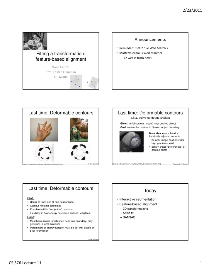
Fitting a transformation: feature-based alignment

Wed, Feb 23

  • Prof. Kristen Grauman

UT‐Austin

Announcements

  • Reminder: Pset 2 due Wed March 2
  • Midterm exam is Wed March 9

(2 weeks from now)

Last time: Deformable contours

Image from http://www.healthline.com/blogs/exercise_fitness/uploaded_images/HandBand2-795868.JPG

Kristen Grauman

Given: initial contour (model) near desired object

a.k.a. active contours, snakes

Figure credit: Yuri Boykov

Goal: evolve the contour to fit exact object boundary

[Snakes: Active contour models, Kass, Witkin, & Terzopoulos, ICCV1987]

Main idea: elastic band is iteratively adjusted so as to

  • be near image positions with

high gradients, and

  • satisfy shape “preferences” or

contour priors

Last time: Deformable contours

Pros:

  • Useful to track and fit non-rigid shapes
  • Contour remains connected
  • Possible to fill in “subjective” contours
  • Flexibility in how energy function is defined, weighted.

Cons:

  • Must have decent initialization near true boundary, may

get stuck in local minimum

  • Parameters of energy function must be set well based on

prior information

Last time: Deformable contours

Kristen Grauman

Today

  • Interactive segmentation
  • Feature-based alignment

– 2D transformations – Affine fit – RANSAC

slide-2
SLIDE 2

2/23/2011 CS 376 Lecture 11 2

Interactive forces

How can we implement such an interactive force with deformable contours?

Kristen Grauman

Interactive forces

  • An energy function can be altered online based
  • n user input – use the cursor to push or pull the

initial snake away from a point.

  • Modify external energy term to include:

 

 

1 2 2

| |

n i i push

p r E 

Nearby points get pushed hardest

Kristen Grauman

Intelligent scissors

[Mortensen & Barrett, SIGGRAPH 1995, CVPR 1999]

Another form of interactive segmentation: Compute optimal paths from every point to the seed based on edge-related costs.

  • http://rivit.cs.byu.edu/Eric/Eric.html

Intelligent scissors

  • http://rivit.cs.byu.edu/Eric/Eric.html

Intelligent scissors

Beyond boundary snapping…

  • Another form of interactive guidance: specify regions
  • Usually taken to suggest foreground/background color

distributions

Boykov and Jolly (2001)

User Input Result How to use this information?

Kristen Grauman

slide-3
SLIDE 3

2/23/2011 CS 376 Lecture 11 3

q

Recall: Images as graphs

Fully-connected graph

  • node for every pixel
  • link between every pair of pixels, p,q
  • similarity wpq for each link

» similarity is inversely proportional to difference in color and position

p wpq

w

Steve Seitz

Recall: Segmentation by Graph Cuts

Break graph into segments

  • Delete links that cross between segments
  • Easiest to break links that have low similarity

– similar pixels should be in the same segments – dissimilar pixels should be in different segments w A B C

Steve Seitz

Link Cut

  • set of links whose removal makes a graph disconnected
  • cost of a cut:

A B Find minimum cut

  • gives you a segmentation
  • fast algorithms exist for doing this

Source: Steve Seitz

 

B q A p q p

w B A cut

, ,

) , (

Recall: Segmentation by Graph Cuts

Adding hard constraints: Add two additional nodes, object and background “terminals” Link each pixel

  • To both terminals
  • To its neighboring pixels

Graph cuts for interactive segmentation

Yuri Boykov

Graph cuts for interactive segmentation

Adding hard constraints: Let the edge weight to

  • bject or background

terminal reflect similarity to the respective seed pixels.

Yuri Boykov Yuri Boykov

Graph cuts for interactive segmentation

Boykov and Jolly (2001)

slide-4
SLIDE 4

2/23/2011 CS 376 Lecture 11 4

Intelligent Scissors Mortensen and Barrett (1995) GrabCut Rother et al. (2004) Graph Cuts Boykov and Jolly (2001)

Graph cuts for interactive segmentation

Another interaction modality: specify bounding box

“Grab Cut”

  • Loosely specify foreground region
  • Iterated graph cut

Rother et al (2004)

User Initialisation

K-means for learning colour distributions Graph cuts to infer the segmentation

?

User initialization

“Grab Cut”

  • Loosely specify foreground region
  • Iterated graph cut

Rother et al (2004)

Gaussian Mixture Model (typically 5-8 components)

Foreground & Background Background Foreground Background

G R G R

Iterated graph cut

“Grab Cut”

Rother et al (2004)

Today

  • Interactive segmentation
  • Feature-based alignment

– 2D transformations – Affine fit – RANSAC

Motivation: Recognition

Figures from David Lowe

slide-5
SLIDE 5

2/23/2011 CS 376 Lecture 11 5

Motivation: medical image registration Motivation: mosaics

Image from http://graphics.cs.cmu.edu/courses/15-463/2010_fal

(In detail next week)

Alignment problem

  • We have previously considered how to fit a model to

image evidence

– e.g., a line to edge points, or a snake to a deforming contour

  • In alignment, we will fit the parameters of some

transformation according to a set of matching feature pairs (“correspondences”). T xi xi

'

Parametric (global) warping

Examples of parametric warps:

translation rotation aspect affine perspective

Source: Alyosha Efros

Parametric (global) warping

Transformation T is a coordinate-changing machine: p’ = T(p) What does it mean that T is global?

  • Is the same for any point p
  • can be described by just a few numbers (parameters)

Let’s represent T as a matrix: p’ = Mp T p = (x,y) p’ = (x’,y’)

             y x y x M ' '

Source: Alyosha Efros

Scaling

Scaling a coordinate means multiplying each of its components by a scalar Uniform scaling means this scalar is the same for all components:

 2

Source: Alyosha Efros

slide-6
SLIDE 6

2/23/2011 CS 376 Lecture 11 6

Non-uniform scaling: different scalars per component:

Scaling

X  2, Y  0.5

Source: Alyosha Efros

Scaling

Scaling operation: Or, in matrix form:

by y ax x   ' '                    y x b a y x ' '

scaling matrix S

Source: Alyosha Efros

What transformations can be represented with a 2x2 matrix?

2D Rotate around (0,0)? y x y y x x * cos * sin ' * sin * cos '        

                        y x y x cos sin sin cos ' '

2D Shear?

y x sh y y sh x x

y x

    * ' * '

                   y x sh sh y x

y x

1 1 ' '

Source: Alyosha Efros

2D Scaling?

y s y x s x

y

x

* ' * '  

                   y x s s y x

y x

' '

What transformations can be represented with a 2x2 matrix?

Source: Alyosha Efros

2D Mirror about Y axis? y y x x

   ' '

                   y x y x 1 1 ' '

2D Mirror over (0,0)? y y x x

    ' '

                     y x y x 1 1 ' '

2D Translation?

y x

t y y t x x     ' '

NO!

2D Linear Transformations

Only linear 2D transformations can be represented with a 2x2 matrix. Linear transformations are combinations of …

  • Scale,
  • Rotation,
  • Shear, and
  • Mirror

                   y x d c b a y x ' '

Source: Alyosha Efros

Homogeneous coordinates

homogeneous image coordinates

Converting from homogeneous coordinates To convert to homogeneous coordinates:

slide-7
SLIDE 7

2/23/2011 CS 376 Lecture 11 7

Homogeneous Coordinates

Q: How can we represent 2d translation as a 3x3 matrix using homogeneous coordinates? A: Using the rightmost column:

           1 1 1

y x

t t ranslation T

y x

t y y t x x     ' '

Source: Alyosha Efros

Translation

                                            1 1 1 1 1 1 ' '

y x y x

t y t x y x t t y x tx = 2 ty = 1 Homogeneous Coordinates

Source: Alyosha Efros

Basic 2D Transformations

Basic 2D transformations as 3x3 matrices

                                    1 1 cos sin sin cos 1 ' ' y x y x                                1 1 1 1 1 ' ' y x t t y x

y x

                               1 1 1 1 1 ' ' y x sh sh y x

y x

Translate Rotate Shear

                               1 1 1 ' ' y x s s y x

y x

Scale

Source: Alyosha Efros

2D Affine Transformations

Affine transformations are combinations of …

  • Linear transformations, and
  • Translations

Parallel lines remain parallel                                w y x f e d c b a w y x 1 ' ' '

Today

  • Interactive segmentation
  • Feature-based alignment

– 2D transformations – Affine fit – RANSAC

Alignment problem

  • We have previously considered how to fit a model to

image evidence

– e.g., a line to edge points, or a snake to a deforming contour

  • In alignment, we will fit the parameters of some

transformation according to a set of matching feature pairs (“correspondences”). T xi xi

'

Kristen Grauman

slide-8
SLIDE 8

2/23/2011 CS 376 Lecture 11 8

Image alignment

  • Two broad approaches:

– Direct (pixel-based) alignment

  • Search for alignment where most pixels agree

– Feature-based alignment

  • Search for alignment where extracted features agree
  • Can be verified using pixel-based alignment

Fitting an affine transformation

  • Assuming we know the correspondences, how do we

get the transformation?

) , (

i i y

x   ) , (

i i y

x

                           

2 1 4 3 2 1

t t y x m m m m y x

i i i i

An aside: Least Squares Example

Say we have a set of data points (X1,X1’), (X2,X2’), (X3,X3’), etc. (e.g. person’s height vs. weight) We want a nice compact formula (a line) to predict X’s from Xs: Xa + b = X’ We want to find a and b How many (X,X’) pairs do we need? What if the data is noisy?

' 2 2 ' 1 1

X b a X X b a X                       

' 2 ' 1 2 1

1 1 X X b a X X Ax=B

                               ... ... ... 1 1 1

' 3 ' 2 ' 1 3 2 1

X X X b a X X X

  • verconstrained

2

min B Ax 

Source: Alyosha Efros

Fitting an affine transformation

  • Assuming we know the correspondences, how do we

get the transformation?

) , (

i i y

x   ) , (

i i y

x

                           

2 1 4 3 2 1

t t y x m m m m y x

i i i i

                                                  

i i i i i i

y x t t m m m m y x y x

2 1 4 3 2 1

1 1

Fitting an affine transformation

  • How many matches (correspondence pairs) do we

need to solve for the transformation parameters?

  • Once we have solved for the parameters, how do we

compute the coordinates of the corresponding point for ?

  • Where do the matches come from?

                                                  

i i i i i i

y x t t m m m m y x y x

2 1 4 3 2 1

1 1

) , (

new new y

x

Kristen Grauman

What are the correspondences?

?

  • Compare content in local patches, find best matches.

e.g., simplest approach: scan with template, and compute SSD

  • r correlation between list of pixel intensities in the patch
  • Later in the course: how to select regions according to

the geometric changes, and more robust descriptors.

Kristen Grauman

slide-9
SLIDE 9

2/23/2011 CS 376 Lecture 11 9

Fitting an affine transformation

Figures from David Lowe, ICCV 1999

Affine model approximates perspective projection of planar objects.

Today

  • Interactive segmentation
  • Feature-based alignment

– 2D transformations – Affine fit – RANSAC

Outliers

  • Outliers can hurt the quality of our parameter

estimates, e.g.,

– an erroneous pair of matching points from two images – an edge point that is noise, or doesn’t belong to the line we are fitting.

Kristen Grauman

Outliers affect least squares fit Outliers affect least squares fit RANSAC

  • RANdom Sample Consensus
  • Approach: we want to avoid the impact of outliers,

so let’s look for “inliers”, and use those only.

  • Intuition: if an outlier is chosen to compute the

current fit, then the resulting line won’t have much support from rest of the points.

slide-10
SLIDE 10

2/23/2011 CS 376 Lecture 11 10

RANSAC: General form

  • RANSAC loop:

1. Randomly select a seed group of points on which to base transformation estimate (e.g., a group of matches) 2. Compute transformation from seed group 3. Find inliers to this transformation 4. If the number of inliers is sufficiently large, re-compute estimate of transformation on all of the inliers

  • Keep the transformation with the largest number of

inliers

RANSAC for line fitting example

Source: R. Raguram

Lana Lazebnik

RANSAC for line fitting example

Least‐squares fit

Source: R. Raguram

Lana Lazebnik

RANSAC for line fitting example

  • 1. Randomly select

minimal subset

  • f points

Source: R. Raguram

Lana Lazebnik

RANSAC for line fitting example

  • 1. Randomly select

minimal subset

  • f points
  • 2. Hypothesize a

model

Source: R. Raguram

Lana Lazebnik

RANSAC for line fitting example

  • 1. Randomly select

minimal subset

  • f points
  • 2. Hypothesize a

model

  • 3. Compute error

function

Source: R. Raguram

Lana Lazebnik

slide-11
SLIDE 11

2/23/2011 CS 376 Lecture 11 11

RANSAC for line fitting example

  • 1. Randomly select

minimal subset

  • f points
  • 2. Hypothesize a

model

  • 3. Compute error

function

  • 4. Select points

consistent with model

Source: R. Raguram

Lana Lazebnik

RANSAC for line fitting example

  • 1. Randomly select

minimal subset

  • f points
  • 2. Hypothesize a

model

  • 3. Compute error

function

  • 4. Select points

consistent with model

  • 5. Repeat

hypothesize‐and‐ verify loop

Source: R. Raguram

Lana Lazebnik 63

RANSAC for line fitting example

  • 1. Randomly select

minimal subset

  • f points
  • 2. Hypothesize a

model

  • 3. Compute error

function

  • 4. Select points

consistent with model

  • 5. Repeat

hypothesize‐and‐ verify loop

Source: R. Raguram

Lana Lazebnik 64

RANSAC for line fitting example

  • 1. Randomly select

minimal subset

  • f points
  • 2. Hypothesize a

model

  • 3. Compute error

function

  • 4. Select points

consistent with model

  • 5. Repeat

hypothesize‐and‐ verify loop

Uncontaminated sample

Source: R. Raguram

Lana Lazebnik

RANSAC for line fitting example

  • 1. Randomly select

minimal subset

  • f points
  • 2. Hypothesize a

model

  • 3. Compute error

function

  • 4. Select points

consistent with model

  • 5. Repeat

hypothesize‐and‐ verify loop

Source: R. Raguram

Lana Lazebnik

RANSAC for line fitting

Repeat N times:

  • Draw s points uniformly at random
  • Fit line to these s points
  • Find inliers to this line among the remaining

points (i.e., points whose distance from the line is less than t)

  • If there are d or more inliers, accept the line

and refit using all inliers

Lana Lazebnik

slide-12
SLIDE 12

2/23/2011 CS 376 Lecture 11 12

RANSAC pros and cons

  • Pros
  • Simple and general
  • Applicable to many different problems
  • Often works well in practice
  • Cons
  • Lots of parameters to tune
  • Doesn’t work well for low inlier ratios (too many iterations,
  • r can fail completely)
  • Can’t always get a good initialization
  • f the model based on the minimum

number of samples

Lana Lazebnik

Today

  • Interactive segmentation
  • Feature-based alignment

– 2D transformations – Affine fit – RANSAC

Coming up: alignment and image stitching