Announcements Lecture #6: Recursion Computer-Science Mentors (CSM) - - PDF document

Announcements

• Computer-Science Mentors (CSM) will be opening section signups

tonight (Monday, Jan. 30) at 8pm. Details will appear on Piazza.

• Starting this Friday, I’ll start a series of extra lectures for those

who want them, 4:30-6:00PM in 306 Soda, covering various topics we don’t have room for. It is completely optional, and is not intended to help you with the course. Sign up for 1 unit of CS198 P/NP under CCN 34691 if interested. To get the unit, attendance required, and a few homeworks.

• HW 2 will be released today. Due next Monday.

Lecture #6: Recursion

Philosophy of Functions (I)

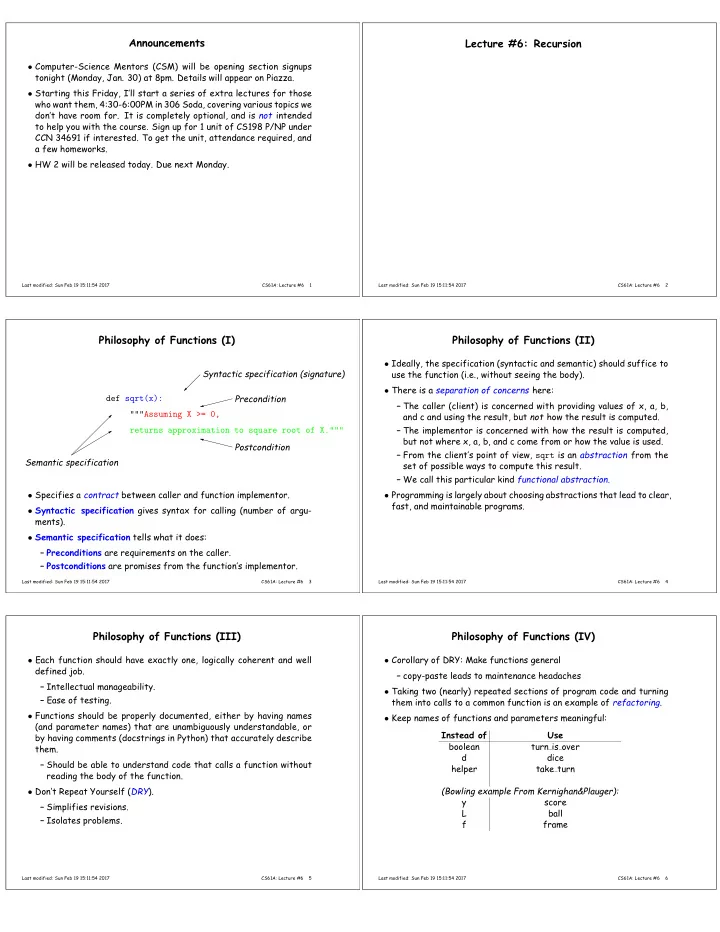
def sqrt(x): """Assuming X >= 0, returns approximation to square root of X.""" Syntactic specification (signature) Precondition Postcondition Semantic specification

• Specifies a contract between caller and function implementor.
• Syntactic specification gives syntax for calling (number of argu-

ments).

• Semantic specification tells what it does:

– Preconditions are requirements on the caller. – Postconditions are promises from the function’s implementor.

Philosophy of Functions (II)

• Ideally, the specification (syntactic and semantic) should suffice to

use the function (i.e., without seeing the body).

• There is a separation of concerns here:

– The caller (client) is concerned with providing values of x, a, b, and c and using the result, but not how the result is computed. – The implementor is concerned with how the result is computed, but not where x, a, b, and c come from or how the value is used. – From the client’s point of view, sqrt is an abstraction from the set of possible ways to compute this result. – We call this particular kind functional abstraction.

• Programming is largely about choosing abstractions that lead to clear,

fast, and maintainable programs.

Philosophy of Functions (III)

• Each function should have exactly one, logically coherent and well

defined job. – Intellectual manageability. – Ease of testing.

• Functions should be properly documented, either by having names

(and parameter names) that are unambiguously understandable, or by having comments (docstrings in Python) that accurately describe them. – Should be able to understand code that calls a function without reading the body of the function.

• Don’t Repeat Yourself (DRY).

– Simplifies revisions. – Isolates problems.

Philosophy of Functions (IV)

• Corollary of DRY: Make functions general

– copy-paste leads to maintenance headaches

• Taking two (nearly) repeated sections of program code and turning

them into calls to a common function is an example of refactoring.

• Keep names of functions and parameters meaningful:

Instead of Use boolean turn is over d dice helper take turn (Bowling example From Kernighan&Plauger): y score L ball f frame

Simple Linear Recursions (Review)

• We’ve been dealing with recursive function (those that call them-

selves, directly or indirectly) for a while now.

• From Lecture #3:

def sum squares(N): """The sum of K**2 for K from 1 to N (inclusive).""" if N < 1: return 0 else: return N**2 + sum squares(N - 1)

• This is a simple linear recursion, with one recursive call per function

instantiation.

• Can imagine a call as an expansion:

sum squares(3) => 3**2 + sum squares(2) => 3**2 + 2**2 + sum squares(1) => 3**2 + 2**2 + 1**2 + sum squares(0) => 3**2 + 2**2 + 1**2 + 0 => 14

• Each call in this expansion corresponds to an environment frame,

linked to the global frame, as shown here.

Tail Recursion

• We’ve also seen a special kind of linear recursion that is strongly

linked to iteration:

def sum squares(N): """The sum of K**2 for 1 <= K <= N.""" accum = 0 k = 1 while k <= N: accum += k**2 k += 1 return accum def sum squares(N): """The sum of K**2 for 1 <= K <= N.""" def part sum(k, accum): if k <= N: return part sum(k+1, accum + k**2) else: return accum part sum(1, 0)

• The right version is a tail-recursive function: the recursive call is

either the returned value or very last action performed.

• The environment frames correspond to the iterations of the loop on

the left, as shown here.

Recursive Thinking

• So far in this lecture, I’ve shown recursive functions by tracing or

repeated expansion of their bodies.

• But when you call a function from the Python library, you don’t look

at its implementation, just its documentation (“the contract”).

• Recursive thinking is the extension of this same discipline to func-

tions as you are defining them.

• When implementing sum squares, we reason as follows:

– Base case: We know the answer is 0 if there is nothing to sum (N < 1). – Otherwise, we observe that the answer is N 2 plus the sum of the positive integers from 1 to N − 1. – But there is a function (sum squares) that can compute 1 + . . . + N − 1 (its comment says so). – So when N ≥ 1, we should return N 2 + sum squares(N − 1).

• This “recursive leap of faith” works as long as we can guarantee we’ll

hit the base case.

Recursive Thinking in Mathematics

• To prevent an infinite recursion, must use this technique only when

– The recursive cases are “smaller” than the input case, and – There is a minimum “size” to the data, and – All chains of progressively smaller cases reach a minimum in a finite number of steps.

• We say that such “smaller than” relations are well founded.
• We have

Theorem (Noetherian Induction): Suppose ≺ is a well-founded relation and P is some property (predicate) such that when- ever P(y) is true for all y ≺ x, then P(x) is also true. Then P(x) is true for all x. (After Emmy Noether 1882–1935, G¨

• ttingen and Bryn Mawr).
• More general than the “line of dominos” induction you may have en-

countered: If true for a base case b, and if true for k when true for k − 1, then true for all k > b.

A Problem

def find first(start, pred): """Find the smallest k >= START such that PRED(START).""" ?

Subproblems and Self-Similarity

• Recursive routines arise when solving a problem naturally involves

solving smaller instances of the same problem.

• A classic example where the subproblems are visible is Sierpinski’s

Triangle (aka bit Sierpinski’s Gasket).

• This triangle may be formed by repeatedly replacing a figure, ini-

tially a solid triangle, with three quarter-sized images of itself (1/2 size in each dimension), arranged in a triangle:

• Or we can think creating a “triangle of order N and size S” by draw-

ing either – a solid triangle with side S if N = 0, or – three triangles of size S/2 and order N −1 arranged in a triangle.

The Gasket in Python

• We can describe this as a recursive Python program that produces

Postscript output.

sin60 = sqrt(3) / 2 def make gasket(x, y, s, n, output): """Write Postscript code for a Sierpinski’s gasket of order N with lower-left corner at (X, Y) and side S on OUTPUT.""" if n == 0: draw solid triangle(x, y, s, output) else: make gasket(x, y, s/2, n - 1, output) make gasket(x + s/2, y, s/2, n - 1, output) make gasket(x + s/4, y + sin60*s/2, s/2, n - 1, output) def draw solid triangle(x, y, s, output): "Draw a solid triangle lower-left corner at (X, Y) and side S." print("{x} {y} moveto " # Go x, y "{s} 0 rlineto " # Horizontal move by s units "-{mid} {alt} rlineto " # Move up and to left "closepath fill" # Close path and fill with black .format(x=x, y=y, s=s, mid=s/2, alt=s*sin60), file=output)

Aside: Using the Functions

• Just to complete the picture, we can use make gasket to create a

standalone Postscript file on a given file.

def draw gasket(n, output=sys.stdout): print("%!", file=output) make gasket(100, 100, 400, 8, output) print("showpage", file=output)

• utput.flush()

# Make sure all output so far is written

• And just for fun, here’s some Python magic to display triangles au-

tomatically (uses gs, the Ghostscript interpreter for Postscript).

from subprocess import Popen, PIPE, DEVNULL def make displayer(): """Create a Ghostscript process that displays its input (sent in through .stdin).""" return Popen("gs", stdin=PIPE, stdout=DEVNULL) >>> d = make displayer() >>> draw gasket(5, d.stdin) >>> draw gasket(10, d.stdin)

Aside: The Gasket in Pure Postscript

• One can also perform the logic to generate figures in Postscript

directly, which is itself a full-fledged programming language:

%! /sin60 3 sqrt 2 div def /make_gasket { dup 0 eq { 3 index 3 index moveto 1 index 0 rlineto 0 2 index rlineto 1 index neg 0 rlineto closepath fill } { 3 index 3 index 3 index 0.5 mul 3 index 1 sub make_gasket 3 index 2 index 0.5 mul add 3 index 3 index 0.5 mul 3 index 1 sub make_gasket 3 index 2 index 0.25 mul add 3 index 3 index 0.5 mul add 3 index 0.5 mul 3 index 1 sub make_gasket } ifelse pop pop pop pop } def 100 100 400 8 make_gasket showpage