An Introduction to 2D Turbulence Jason Laurie Mathematics Group - - PowerPoint PPT Presentation

An Introduction to 2D Turbulence

Jason Laurie

Mathematics Group School of Engineering and Applied Science Aston University

Waves, coherent structures, and turbulence, UEA, 30th October 2019

Outline

• Key results of 3D turbulence
• 2D turbulence theory
• Experiments and simulations
• Energy condensation and mean flows
• Thin layer turbulence: 2D to 3D transition

Why is 2D turbulence important?

Mean flows in geophysical turbulence Thin-layer fluid experiments

Sommeria,

• J. Fluid Mech. 170,

139, (1986)

Why is 2D turbulence important?

• Stable large-scale coherent mean flow
• Typically generated out of small-scale

fluctuations

• In non-equilibrium balance between

forcing and dissipation

Mean flows in geophysical turbulence Properties Thin-layer fluid experiments

Navier-Stokes and turbulence

3D Navier-Stokes equations

∂v ∂t + (v · r) v = 1 ρrp + νr2v + f

Increasing

• Ratio of the nonlinear advection term to

that of viscous diffusion

Turbulence appears when 1 ⌧ Re

Re ' 26 Re ' 2000 Re ' 1.54

Re

Osbourne Reynolds (1883)

Re = |(v · r)v| |νr2v| ⇠ V L ν

Claude-Louis Navier and George Stokes (1827-1845)

Reynolds number r · v = 0

The Navier-Stokes equation

3D Navier-Stokes equations

∂v ∂t + (v · r) v = 1 ρrp + νr2v + f

Claude-Louis Navier and George Stokes (1827-1845)

r · v = 0 The energy balance equation

• In the inviscid limit, the Navier-Stokes equation conserves the kinetic energy

Z = 1 2 Z |r ⇥ v|2 dx

E = 1 2 Z |v|2 dx

Kinetic Energy Enstrophy

dE dt = −2⌫Z = −✏

Dissipative anomaly

✏ = lim

ν→0 2⌫Z > 0

• However, in the inviscid limit, experimentally the

energy dissipation rate remains finite

✏

• Inertial range dynamics: scale separation

between forcing and dissipation

• Under the assumptions of scale

invariance, isotropy, and homogeneity Kolmogorov proved that for the velocity increments

Kolmogorov’s theory for turbulence

Richardson’s cascade picture

“Big whirls have little whirls that feed on their velocity, and little whirls have lesser whirls and so on to viscosity.”

Lewis Fry Richardson, Weather Prediction by Numerical Process, (1922)

Kolmogorov’s four-fifths law h(vr)3i = 4 5✏r

δvr(x) = [v(x + r) − v(x)] · r

• A. N. Kolmogorov, Dokl. Akad. Nauk SSSR 30, 299 (1941)

• A ‘universal’ dimensionless prefactor for

is experimentally measure to be around

Ek = C✏2/3k−5/3

Kolmogorov’s energy spectrum

Kolmogorov’s Energy Spectrum

• Distribution of energy in scale-space can be observe by computing

the 1D energy spectrum defined through

h(vr)3i = 4 5✏r E = 1 2 Z

D

|v|2 dr = Z Ek dk

Ek

• Assuming we satisfy Kolmogorov’s four-fifths law
• Then, by dimensional arguments the second order

velocity increment correlator scales as

h(vr)2i / ✏2/3r2/3 ⇒ Ek ∝ ✏2/3k−5/3 k−5/3

• A. N. Kolmogorov, Dokl. Akad. Nauk SSSR 30, 299 (1941)
• A. M Obukhov, Dokl. Akad. Nauk SSSR, 5, 453–466, (1941)

C ' 1.5

Turbulence intermittency

Structure function scaling from K41

• From the assumptions of Kolmogorov K41 theory, we expect that

the statistical moments of turbulent velocity structure functions should scale as

h(vr)pi = Cn (✏r)p/3

Intermittency

• Strong deviations from K41 for
• Several models have been proposed

to explain the deviation from

• Intermittency is related to velocity

phase correlations

ζp = p/3

p > 3

Leveque and She, (1993) Frisch, (1995)

Outline 2D Turbulence Theory and Experiments

Thin-layer fluid flows

Thin-layer approximation: 2D Navier-Stokes with linear friction

r · v = 0

Consider a thin-layer fluid flow governed by 3D Navier-Stokes equations

• Neglect vertical motions because
• Assume a Poiseuille velocity profile in the vertical direction u(z), v(z) ∝ z2

r · v = 0 v = (u, v) v = (u, v, w) ∂v ∂t + (v · r) v = rp + νr2v + f ∂v ∂t + (v · r) v = rp + νr2v αv + f w ∼ O(h/L)(u, v)

νr2

(3D)v

! νr2

(2D)v αv

Ekman friction (rotating flows) Rayleigh friction (stratified flows) Hartmann friction (MHD) Air friction (soap films)

α ∼ O(ν/h2)

{

α

The 2D Navier-Stokes equations

The 2D Navier-Stokes is the simplest turbulence model for the large-scale motion of geophysical flows where rotation, stratification, or thin-layers suppresses vertical motions

∂ω ∂t + v · rω = νr2ω αω + fω v = ez ⇥ rψ ω = r2ψ Vorticity formalism of 2D Navier-Stokes 2D Navier-Stokes has an infinite number of inviscid invariants E = 1 2 Z

D

|v|2 dr Energy Casimir Functionals Cf = Z

D

f(ω) dr

ω = (r ⇥ v) · ez

Energy balance in 2D

No energy dissipative anomaly in 2D Palinstrophy Z = 1 2 Z

D

ω2 dr Enstrophy

Of all the invariants, energy and enstrophy are the most important

E = 1 2 Z

D

|v|2 dr Energy Energy and Enstrophy balance equations dE dt = −2νZ

dZ dt = −2νP

P = 1 2 Z |r ⇥ ω|2 dr

lim

ν→0

dE dt = 0

• As the enstrophy remains bounded, the energy dissipation rate cannot remain

finite in the inviscid limit

• As the palinstrophy is positive definite, the total enstrophy cannot grow

2D turbulent cascades

Two quadratic invariants imply a double cascade Fjørtoft, Tellus, 5, 225, (1953)

• Assume there exists two sinks and one source separated by two inertial ranges

Ek k

✏I = ✏α + ✏ν ηI = ηα + ην l2

α = ✏α/⌘α

l2

ν = ✏ν/⌘ν

l2

I = ✏I/⌘I

✏I ηI ηα ✏α ✏ν ην

Stationary state Enstrophy ratio Energy ratio

✏ν ✏α = ✓lν lI ◆2 1 − (lI/lα)2 1 − (lν/lI)2

lν⌧lI⌧lα

− − − − − − − → 0

lν⌧lI⌧lα

− − − − − − − → 0

Energy E n s t r

• p

h y

ηα ην = ✓ lI lα ◆2 1 − (lν/lI)2 1 − (lI/lα)2

Characteristic scales

• Total enstrophy divergences in large

wavenumber limit: nonlocality

• Proposed a logarithmic correction to imply

convergence

2D energy spectra

Kraichnan-Leith-Batchelor phenomenology

h(vr)3i = 3 2✏r hδvr (δωr)2i = 2ηr

Inverse energy cascade Direct enstrophy cascade

h(vr)2i / ✏2/3r2/3 ) Ek / ✏2/3k−5/3 h(δvr)2i / η2/3r2 ) Ek / η2/3k−3

Kraichnan’s logarithmic correction

Ek ∝ η2/3k−3 ln−1/3 (kL)

k Ek

E

k

∝ η

2 / 3

k

− 3

ln

− 1 / 3

(kL)

Ek ∝ ✏2/3k−5/3

Energy spectrum scalings

• Following the results of Kolmogorov for 3D turbulence, it

is possible to obtain equivalent results for 2D turbulence

(1967-1969) Lindborg, J. Fluid Mech. 355, 259-288, (1999) (1971)

Evidence from atmospheric data

Nastrom et al. Nature, 312, (1984)

GASP aircraft data of wind speeds in tropopause

k−5/3

• bserved for

wavelength 3-300km

k−5/3

Experimental evidence: soap films

Cerbus and Goldburg. Phys. Fluids, 25, (2013)

Soap film experiments

Couder, Goldburg, Kellay, Rutgers, Rivera, Ecke,…

Experimental evidence: thin-layer fluids

Paret and Tabeling. Phys. Rev. Lett. 79, 4162, (1997)

Thin layer electrolytes driven by a Lorenz force Sommeria, Tabeling, Gollub, Shats,…

Numerical evidence

Enstrophy Flux 2D Navier-Stokes with linear friction

Boffetta and Musacchio,

• Phys. Rev. E, 82, 016307, (2010)

Forcing Energy Flux ∂ω ∂t + v · rω = νr2ω αω + fω

2D structure functions

Third order structure function

Inverse energy cascade Direct enstrophy cascade

Boffetta and Musacchio, Phys. Rev. E, 82, 016307, (2010)

D (vr)3E = 8 > > > < > > > : 1 8⌘r3 for r ⌧ lf 3 2✏r for lf ⌧ r

Higher order structure functions Boffetta, Celani and Vergassola, Phys. Rev. E, 61, 29, (2000)

Structure function scalings compatible with - no intermittency!

h(vr)pi / (✏r)p/3

Outline 2D Energy Condensation and Large-Scale Mean Flows

Energy condensation in 2D

Realizability of the inverse cascade of energy

• Infinite sized systems
• Finite size with sufficient large-scale dissipation

Otherwise…spectral condensation

• Inverse cascade reaches the largest scale and is blocked
• Energy will continuously be fed into the largest modes
• Observed behaviour

Chertkov et al.

• Phys. Rev. Lett.

99, 084501, (2007)

Ek ∝ k−3

Energy Spectrum Energy Flux Forced 2D Navier-Stokes without linear friction

Energy condensation in 2D

Spectral condensation leads to spatial self-organization of the flow

Chertkov et al. Phys. Rev. Lett. 99, 084501, (2007) van Heijst et al. J. Fluid Mech. 554, 411, (2006)

Periodic boundaries No-slip boundaries

• Form of mean flow is dependent on domain and boundary conditions

2D Navier-Stokes simulations

Energy condensation in experiments

Shats et al.

• Phys. Rev. E, 71,

046409, (2005)

• Argument justified for dynamical systems relaxing toward equilibrium (Euler dynamics)
• is the local probability to have at position

How to predict the condensate?

Equilibrium statistical mechanics: Miller-Robert-Sommeria (1990, 1991)

ω(r) = Ω r ρ(r, Ω)

Microcanonical variational problem

S(E, γ) = sup

ρ

⇢Z Z ∞

−∞

ρ ln ρ dΩ dr | E[ρ] = E, D[ρ] = γ

• Energy-Casimir variational problem
• In principle this extremely tough problem
• Solutions of the EC-VP are solutions of the MVP for the particular energy and casimirs

C(E, s) = inf

ω

⇢ Cs[ω] = Z

D

s(ω) dr | E[ω] = E

• However, it can be shown that entropy maximisers satisfy

ω = f(βψ) ) v · rω = 0

Miller, Phys. Rev. Lett. 65, 2137, (1990) Robert, Sommeria, J. Fluid Mech. 229, 291, (1991)

How to predict the condensate?

Energy-Casimir variational problem Solution in the weak energy limit

C(E, s) = inf

ω

⇢ Cs[ω] = Z

D

s(ω) dr | E[ω] = E

• At leading order, enstrophy becomes the most

important casimir and we get a linear relationship

• Leads to largest-scale argument where energy is

situated at the eigenmodes with smallest eigenvalue

• Degeneracy is removed by considering next order

casimir or aspect ratios > 1

ω = A cos(x) + B cos(y)

Bouchet and Venaille, Phys. Rep. 515, 227 (2012)

s(ω) = ω2 2 + a4ω4 4 + o(ω5)

ω = βψ

Decaying 2D Navier-Stokes turbulence

Dipole appears at largest scale as flow decays

Matthaeus et al. Physica D, 51, 531, (1991)

Numerics Theory

ω = A cos(x) + B cos(y)

Forced 2D Navier-Stokes turbulence

Bouchet and Simonnet, Phys. Rev. Lett. 102, 094504, (2009)

• Both dipole and zonal jets appear depending on the aspect ratio of periodic domain
• Vorticity-Streamfunction relation is nonlinear:

Stochastically forced 2D Navier-Stokes with linear friction Mean flow not solely contained in largest modes

• Mean vorticity scaling appears to be
• Largest scale argument is insufficient to predict profile: does not lead to
• A non-equilibrium approach is likely needed to explain mean flow structure

Vortex profile in forced 2D turbulence

Chertkov et al. Phys. Rev. Lett. 99, 084501, (2007) Xia et al. Phys. Fluids, 21, 125101, (2009)

2D Navier-Stokes equations Thin-layer experiment Observations

Ω ∝ r−5/4 Ω ∝ r−5/4

Mean flow energy/momentum balance

Reynolds flow decomposition v = (vφ, vr) = (U(r) + u(φ, r, t), v(φ, r, t)) hvi = (U(r), 0) hui = hvi = 0

• Decompose flow into its temporal mean and fluctuating

components using polar coordinates

vr

vφ

1 r ∂r

• r2huvi
• = αrU

Momentum balance ∂rhrv2i + r∂rhpi = U 2 + hu2i radial component azimuthal component Energy balance

1 r ∂r (rUhuvi) = rhuvi∂r ✓U r ◆ αU 2

1 r @r  r ⌧ v ✓u2 + v2 2 + p ◆ = ✏ ↵hu2 + v2i rhuvi@r ✓U r ◆

Energy balance

• f mean flow

Energy balance

• f fluctuations

Vortex profile prediction

1 r ∂r

• r2huvi
• = αrU

Energy balance Momentum balance (azimuthal component) ✏ = 1 r @r (rUhuvi) + ↵U 2 U = p 3✏/↵ Ω = p 3✏/↵ r−1 huvi = r↵✏ 3 r 1 r @r (rUhuvi) = 2✏

• Not only scaling, but also numerical prefactors are predicted!
• Notice the shallower mean vorticity scaling to what was previously observed

JL et al. Phys. Rev. Lett. 113, 254503, (2014)

Power-law solutions of energy and momentum balance equations Neglect higher-order turbulent velocity correlators

• We have a natural small parameter that relates the strength of the

mean flow shear to that of the turbulence fluctuations

• Further assume that can also be neglected inside vortex

↵3L2/✏ ⌧ 1 hvpi

Mean vortex velocity data

100 101 102 103 10−2 10−1

αL2/ 1/2 Ω

r/L A B C D √ 3 (r/L)−1 0.5 1 1.5 2 2.5 10−2 10−1 (α/)1/2 U r/L A B C D √ 3

Mean vorticity profile Mean azimuthal velocity profile U = p 3✏/↵ Ω = p 3✏/↵ r−1

JL et al. Phys. Rev. Lett. 113, 254503, (2014)

α

Numerical simulations

• Forced/dissipated pseudo-spectral simulations with small-

scale forcing

• Simulations A-C have spatial resolution 5122, while simulation

D is 10242

• All simulations have different linear friction coefficient

Condensates in rectangular domains

Energy condensates in rectangular domains

• A. Frishman, JL, G. Falkovich, Phys. Rev. Fluids, 2, 032602, (2017)

−0.5 0.5 −0.5 0.5 −0.5 0.5 −0.5 0.5 y/L x/(lxL) −0.5 0.5 −0.5 0.5 −80 80 (a) y/L x/(lxL) −0.5 0.5 −0.5 0.5 −20 20 (b) −0.5 0.5 −0.5 0.5 −0.5 0.5 −0.5 0.5 y/L x/(lxL) −0.5 0.5 −0.5 0.5 −80 80 (a) x/(lxL) −0.5 0.5 −0.5 0.5 −20 20 (b)

= ✓ ↵3 ✏L2 ◆1/3

δ = 1.1 × 10−2 δ = 2.8 × 10−3

Temporal mean displays zonal symmetry

Zonal jet profile

U(y) = r 2✏ ↵ InvErf ✓2y ⇡ ◆

Jet profile prediction

• Both balance equations imply any solution must satisfy

which cannot be satisfied when because must remain finite

@yUhuvi = ✏

∂yU ≈ 0

huvi

Momentum and energy balance for zonal state The closure cannot remain valid in the whole domain

−2 −1.5 −1 −0.5 0.5 1 1.5 2 −0.5 −0.25 0.25 0.5

• α/ U

y/L

• α/ U

Theory −2 −1.5 −1 −0.5 0.5 1 1.5 2 −0.5 −0.25 0.25 0.5

• α/ U

y/L

• α/ U

Theory

• A. Frishman, JL, G. Falkovich, Phys. Rev. Fluids, 2, 032602, (2017)

vortices vortices

Assumptions satisfied

∂yhuvi = αU

Outline Thin Layer Turbulence: 2D to 3D Transition

Phenomenology of quasi-2D flows

Lx

Ly

Lz

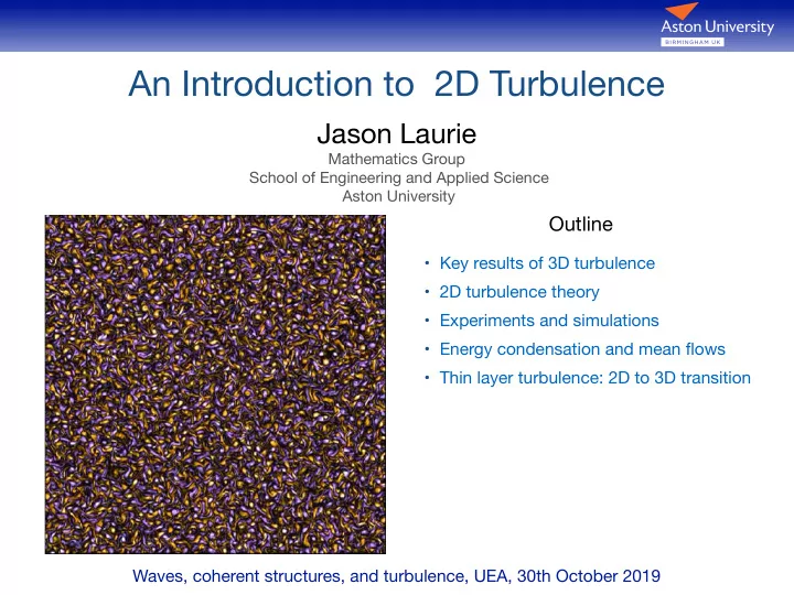
Transition from 2D to 3D turbulence as thickness increases Lz

2D inverse cascade 3D direct cascade ?

∂v ∂t + (v · r) v = 1 ρrp + νr2v + f

r · v = 0 3D Navier-Stokes equations

Celani et al. Phys. Rev. Lett. 104, 184506, (2010) Musacchio and Boffetta, Phys. Fluids, 29, 111106, (2017) Musacchio and Boffetta, Phys. Rev. Fluids, 4, 022602(R), (2019)

• Most real 2D flows are quasi-2D, e.g. the height of Earth’s

atmosphere is ~100km, while the circumference is ~40,000km

0 < Lz < lν < Lf < Lx, Ly

0 < lν < Lz < Lf < Lx, Ly

0 < lν < Lf < Lz < Lx, Ly

Energy growth as 2D becomes 3D

Numerical simulations of quasi-2D turbulence

• In pure 2D, energy grows linear in time
• The energy growth rate decreases as the thickness increases
• For observed energy growth rate = rate of energy injection
• For energy growth rate vanishes

Lz < lν

lν < Lf/2 < Lz

Celani et al. Phys. Rev. Lett. 104, 184506, (2010)

2D 3D

Split energy cascade

Coexisting inverse and direct energy cascades

2D 3D 3D 2D

Lz Lf = 1 4

0 < lν < Lz < Lf < Lx

• In the transition region, part of the energy is transferred to large-scales via a 2D

inverse cascade, while the rest goes to small-scales via a 3D direct cascade

Celani et al. Phys. Rev. Lett. 104, 184506, (2010)

Summary

• 2D Navier-Stokes is the simplest model for geophysical flows
• 2D turbulence is a dual-cascade system
• The inverse energy cascade leads to energy condensation
• Mathematical Prediction of large-scale mean flows
• Quasi 2D turbulence: 2D - 3D transition
• What I didn’t mention: conformal invariance; bistability; 2D

geophysical turbulence;…