Algoritmi di Bioinformatica Zsuzsanna Lipt ak Laurea Magistrale - - PDF document

Algoritmi di Bioinformatica

Zsuzsanna Lipt´ ak

Laurea Magistrale Bioinformatica e Biotechnologie Mediche (LM9) a.a. 2014/15, spring term

Computational efficiency I

2 / 18

Computational Efficiency

As we will see later in more detail, the efficiency of algorithms is measured w.r.t.

• running time
• storage space

We will make these concepts more concrete later on, but for now want to give some intuition, using an example.

3 / 18

Example: Computation of nth Fibonacci number

Fibonacci numbers: model for growth of populations (simplified model)

• Start with 1 pair of rabbits in a field
• each pair becomes mature at age of 1 month and mates
• after gestation period of 1 month, a female gives birth to 1 new pair
• rabbits never die1

Definition

F(n) = number of pairs of rabbits in field at the beginning of the n’th month.

1This unrealistic assumption simplifies the mathematics; however, it turns out that

adding a certain age at which rabbits die does not significantly change the behaviour of the sequence, so it makes sense to simplify.

4 / 18

Computation of nth Fibonacci number

• month 1: there is 1 pair of rabbits in the field

F(1) = 1

• month 2: there is still 1 pair of rabbits in the field

F(2) = 1

• month 3: there is the old pair and 1 new pair

F(3) = 1 + 1 = 2

• month 4: the 2 pairs from previous month, plus

the old pair has had another new pair F(4) = 2 + 1 = 3

• month 5: the 3 from previous month, plus

the 2 from month 3 have each had a new pair F(5) = 3 + 2 = 5

Recursion for Fibonacci numbers

F(1) = F(2) = 1 for n > 2: F(n) = F(n − 1) + F(n − 2).

5 / 18

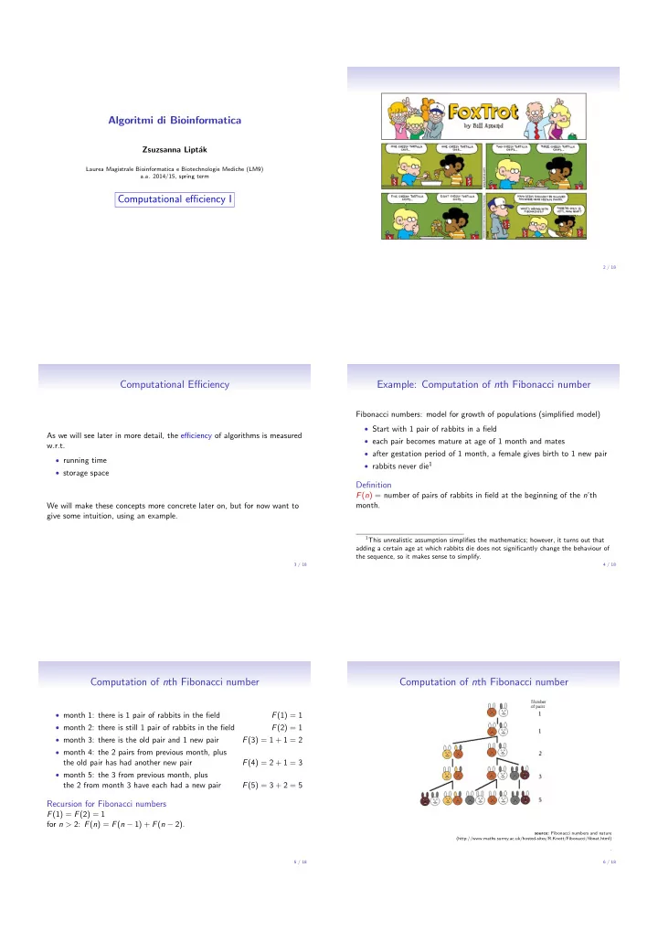
Computation of nth Fibonacci number

source: Fibonacci numbers and nature (http://www.maths.surrey.ac.uk/hosted-sites/R.Knott/Fibonacci/fibnat.html) . 6 / 18

Computation of nth Fibonacci number

The first few terms of the Fibonacci sequence are: n 1 2 3 4 5 6 7 8 9 10 11 12 13 14 F(n) 1 1 2 3 5 8 13 21 34 55 89 144 233 377 n 15 16 17 18 19 20 21 22 23 F(n) 610 987 1 597 2 584 4 181 6 765 10 946 17 711 28 657

7 / 18

Fibonacci numbers in nature

21 spirals left 34 spirals right

source: Plant Spiral Exhibit (http://cs.smith.edu/ phyllo/Assets/Images/ExpoImages/ExpoTour/index.htm) On these pages it is explained how these plants develop. Very interesting! 8 / 18

Fibonacci numbers in nature

8 spirals left 13 spirals right

source: Plant Spiral Exhibit (http://cs.smith.edu/ phyllo/Assets/Images/ExpoImages/ExpoTour/index.htm) . 9 / 18

Fibonacci numbers in nature

21 spirals left 13 spirals right

source: Fibonacci numbers and nature (http://www.maths.surrey.ac.uk/hosted-sites/R.Knott/Fibonacci/fibnat.html) very nice page! recommended! 10 / 18

Growth of Fibonacci numbers

Theorem

For n > 6: F(n) > (1.5)n−1.

Proof:

Note that from n = 3 on, F(n) strictly increases, so for n ≥ 4, we have F(n − 1) > F(n − 2). Therefore, F(n − 1) > 1

2F(n).

We prove the theorem by induction: Base: For n = 6, we have F(6) = 8 > 7.59 . . . = (1.5)5. Step: Now we want to show that F(n + 1) > (1.5)n. By the I.H. (induction hypothesis), we have that F(n) > (1.5)n−1. Since F(n − 1) > 0.5F(n), it follows that F(n + 1) = F(n) + F(n − 1) > 1.5 · F(n) > (1.5) · (1.5)n−1 = (1.5)n.

11 / 18

Computation of nth Fibonacci number

Algorithm 1 (let’s call it fib1) works exactly along the recursive definition: Algorithm fib1(n) 1. if n = 1 or n = 2 2. then return 1 3. else 4. return fib1(n − 1) + fib1(n − 2)

12 / 18

Computation of nth Fibonacci number

Analysis

(sketch) Looking at the computation tree, we can see that the tree for computing F(n) has F(n) many leaves (show by induction), where we have a lookup for F(2) or F(1). A binary rooted tree has one fewer internal nodes than leaves (see second part of course, or show by induction), so this tree has F(n) − 1 internal nodes, each of which entails an addition. So for computing F(n), we need F(n) lookups and F(n) − 1 additions, altogether 2F(n) − 1 operations (additions, lookups etc.). The algorithm has exponential running time, since it makes 2F(n) − 1, i.e. at least 2 · (1.5)n−1 − 1 steps (operations).

13 / 18

Computation of nth Fibonacci number

Algorithm 2 (let’s call it fib2) computes every F(k), for k = 1 . . . n, iteratively (one after another), until we get to F(n). Algorithm fib2(n) 1. array of int F[1 . . . n]; 2. F[1] ← 1; F[2] ← 1; 3. for k = 3 . . . n 4. do F[k] ← F[k − 1] + F[k − 2]; 5. return F[n];

Analysis

(sketch) One addition for every k = 1, . . . , n. Uses an array of integers of length n.—The algorithm has linear running time and linear storage space.

14 / 18

Computation of nth Fibonacci number

Algorithm 3 (let’s call it fib3) computes F(n) iteratively, like Algorithm 2, but using only 3 units of storage space. Algorithm fib3(n) 1. int a, b, c; 2. a ← 1; b ← 1; c ← 1; 3. for k = 3 . . . n 4. do c ← a + b; 5. a ← b; b ← c; 6. return c;

Analysis

(sketch) Time: same as Algo 2. Uses 3 units of storage (called a, b, and c).—The algorithm has linear running time and constant storage space.

15 / 18

Comparison of running times

n 1 2 3 4 5 6 7 10 20 30 40 F(n) 1 1 2 3 5 8 13 55 6 765 832 040 102 334 155 fib1 1 1 3 5 9 15 25 109 13 529 1 664 079 204 668 309 fib2 1 2 3 4 5 6 7 10 20 30 40 fib3 1 2 3 4 5 6 7 10 20 30 40 The number of steps each algorithm makes to compute F(n).

16 / 18

Summary

• We saw 3 different algorithms for the same problem (computing the

nth Fibonacci number).

• They differ greatly in their efficiency:
• Algo fib1 has exponential running time.
• Algo fib2 has linear running time and linear storage space.
• Algo fib3 has linear running time and constanct storage space.
• We saw on an example computation (during class) that exponential

running time is not practicable.

17 / 18

Summary (2)

Take-home message

• There may be more than one way of computing something.
• It is very important to use efficient algorithms.
• Efficiency is measured in terms of running time and storage space.
• Computation time is important for obvious reasons: the faster the

algorithm, the more problems we can solve in the same amount of time.

• In computational biology, inputs are often very large, therefore storage

space is at least as important as running time.

18 / 18