Algorithmic Paradigms Greedy. Build up a solution incrementally, - PowerPoint PPT Presentation

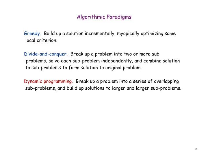
Algorithmic Paradigms Greedy. Build up a solution incrementally, myopically optimizing some local criterion. Divide-and-conquer. Break up a problem into two or more sub -problems, solve each sub-problem independently, and combine solution to sub-problems to form solution to original problem. Dynamic programming. Break up a problem into a series of overlapping sub-problems, and build up solutions to larger and larger sub-problems. 2

Dynamic Programming History Bellman. Pioneered the systematic study of dynamic programming in the 1950s. Etymology.  Dynamic programming = planning over time.  Secretary of Defense was hostile to mathematical research.  Bellman sought an impressive name to avoid confrontation. – "it's impossible to use dynamic in a pejorative sense" – "something not even a Congressman could object to" Reference: Bellman, R. E. Eye of the Hurricane, An Autobiography. 3

Dynamic Programming Applications Areas.  Bioinformatics.  Control theory.  Information theory.  Operations research.  Computer science: theory, graphics, AI, systems, …. Some famous dynamic programming algorithms.  Viterbi for hidden Markov models.  Unix diff for comparing two files.  Smith-Waterman for sequence alignment.  Bellman-Ford for shortest path routing in networks.  Cocke-Kasami-Younger for parsing context free grammars. 4

6.1 Weighted Interval Scheduling

Weighted Interval Scheduling Weighted interval scheduling problem.  Job j starts at s j , finishes at f j , and has weight or value v j .  Two jobs compatible if they don't overlap.  Goal: find maximum weight subset of mutually compatible jobs. a b c d e f g h Time 0 1 2 3 4 5 6 7 8 9 10 11 6

Unweighted Interval Scheduling Review Recall. Greedy algorithm works if all weights are 1.  Consider jobs in ascending order of finish time.  Add job to subset if it is compatible with previously chosen jobs. Observation. Greedy algorithm can fail spectacularly if arbitrary weights are allowed. b weight = 999 a weight = 1 Time 0 1 2 3 4 5 6 7 8 9 10 11 7

Weighted Interval Scheduling Notation. Label jobs by finishing time: f 1 ≤ f 2 ≤ . . . ≤ f n . Def. p(j) = largest index i < j such that job i is compatible with j. Ex: p(8) = 5, p(7) = 3, p(2) = 0. 1 2 3 4 5 6 7 8 Time 0 1 2 3 4 5 6 7 8 9 10 11 8

Dynamic Programming: Binary Choice Notation. OPT(j) = value of optimal solution to the problem consisting of job requests 1, 2, ..., j.  Case 1: OPT selects job j. – can't use incompatible jobs { p(j) + 1, p(j) + 2, ..., j - 1 } – must include optimal solution to problem consisting of remaining compatible jobs 1, 2, ..., p(j) optimal substructure  Case 2: OPT does not select job j. – must include optimal solution to problem consisting of remaining compatible jobs 1, 2, ..., j-1  0 if j = 0 OPT ( j ) =  v j + OPT ( p ( j )), OPT ( j − 1) { } max otherwise  9

Weighted Interval Scheduling: Brute Force Brute force algorithm. Input: n, s 1 ,…,s n , f 1 ,…,f n , v 1 ,…,v n Sort jobs by finish times so that f 1 ≤ f 2 ≤ ... ≤ f n . Compute p(1), p(2), …, p(n) Compute-Opt(j) { if (j = 0) return 0 else return max(v j + Compute-Opt(p(j)), Compute-Opt(j-1)) } 10

Weighted Interval Scheduling: Brute Force Observation. Recursive algorithm fails spectacularly because of redundant sub-problems ⇒ exponential algorithms. Ex. Number of recursive calls for family of "layered" instances grows like Fibonacci sequence. 5 4 3 1 2 3 2 2 1 3 4 2 1 1 1 5 1 p(1) = 0, p(j) = j-2 11

Weighted Interval Scheduling: Memoization Memoization. Store results of each sub-problem in a cache; lookup as needed. Input: n, s 1 ,…,s n , f 1 ,…,f n , v 1 ,…,v n Sort jobs by finish times so that f 1 ≤ f 2 ≤ ... ≤ f n . Compute p(1), p(2), …, p(n) for j = 1 to n global array M[j] = empty M[j] = 0 M-Compute-Opt(j) { if (M[j] is empty) M[j] = max(w j + M-Compute-Opt(p(j)), M-Compute-Opt(j-1)) return M[j] } 12

Weighted Interval Scheduling: Running Time Claim. Memoized version of algorithm takes O(n log n) time.  Sort by finish time: O(n log n).  Computing p( ⋅ ) : O(n) after sorting by start time. M-Compute-Opt(j) : each invocation takes O(1) time and either  – (i) returns an existing value M[j] – (ii) fills in one new entry M[j] and makes two recursive calls  Progress measure Φ = # nonempty entries of M[] . – initially Φ = 0, throughout Φ ≤ n. – (ii) increases Φ by 1 ⇒ at most 2n recursive calls.  Overall running time of M-Compute-Opt(n) is O(n). ▪ 13

Automated Memoization Automated memoization. Many functional programming languages (e.g., Lisp) have built-in support for memoization. Q. Why not in imperative languages (e.g., Java)? static int F(int n) { (defun F (n) if (n <= 1) return n; (if else return F(n-1) + F(n-2); (<= n 1) } n (+ (F (- n 1)) (F (- n 2))))) Java (exponential) Lisp (efficient) F(40) F(39) F(38) F(38) F(37) F(37) F(36) F(37) F(36) F(36) F(35) F(36) F(35) F(35) F(34) 14

Weighted Interval Scheduling: Finding a Solution Q. Dynamic programming algorithms computes optimal value. What if we want the solution itself? A. Do some post-processing. Run M-Compute-Opt(n) Run Find-Solution(n) Find-Solution(j) { if (j = 0) output nothing else if (v j + M[p(j)] > M[j-1]) print j Find-Solution(p(j)) else Find-Solution(j-1) }  # of recursive calls ≤ n ⇒ O(n). 15

Weighted Interval Scheduling: Bottom-Up Bottom-up dynamic programming. Unwind recursion. Input: n, s 1 ,…,s n , f 1 ,…,f n , v 1 ,…,v n Sort jobs by finish times so that f 1 ≤ f 2 ≤ ... ≤ f n . Compute p(1), p(2), …, p(n) Iterative-Compute-Opt { M[0] = 0 for j = 1 to n M[j] = max(v j + M[p(j)], M[j-1]) } 16

6.3 Segmented Least Squares

Segmented Least Squares Least squares.  Foundational problem in statistic and numerical analysis.  Given n points in the plane: (x 1 , y 1 ), (x 2 , y 2 ) , . . . , (x n , y n ).  Find a line y = ax + b that minimizes the sum of the squared error: y n ( y i − ax i − b ) 2 SSE = ∑ i = 1 x Solution. Calculus ⇒ min error is achieved when y i − a x i a = n x i y i − ( x i ) y i ) ( ∑ ∑ ∑ ∑ ∑ i i i i i b = , 2 − ( n x i ) 2 n x i ∑ ∑ i i 18

Segmented Least Squares Segmented least squares.  Points lie roughly on a sequence of several line segments.  Given n points in the plane (x 1 , y 1 ), (x 2 , y 2 ) , . . . , (x n , y n ) with  x 1 < x 2 < ... < x n , find a sequence of lines that minimizes f(x). Q. What's a reasonable choice for f(x) to balance accuracy and parsimony? goodness of fit number of lines y x 19

Segmented Least Squares Segmented least squares.  Points lie roughly on a sequence of several line segments.  Given n points in the plane (x 1 , y 1 ), (x 2 , y 2 ) , . . . , (x n , y n ) with  x 1 < x 2 < ... < x n , find a sequence of lines that minimizes: – the sum of the sums of the squared errors E in each segment – the number of lines L  Tradeoff (penalty) function: E + c L, for some constant c > 0. y x 20

Dynamic Programming: Multiway Choice Notation.  OPT(j) = minimum cost for points p 1 , p i+1 , . . . , p j .  e(i, j) = minimum sum of squares for points p i , p i+1 , . . . , p j . To compute OPT(j):  Last segment uses points p i , p i+1 , . . . , p j for some i.  Cost = e(i, j) + c + OPT(i-1).  0 if j = 0  OPT ( j ) =  e ( i , j ) + c + OPT ( i − 1) min { } otherwise   1 ≤ i ≤ j 21

Segmented Least Squares: Algorithm INPUT: n, p 1 ,…,p N , c Segmented-Least-Squares() { M[0] = 0 for j = 1 to n for i = 1 to j compute the least square error e ij for the segment p i ,…, p j for j = 1 to n M[j] = min 1 ≤ i ≤ j (e ij + c + M[i-1]) return M[n] } can be improved to O(n 2 ) by pre-computing various statistics Running time. O(n 3 ).  Bottleneck = computing e(i, j) for O(n 2 ) pairs, O(n) per pair using previous formula. 22