Alex Psomas: Lecture 15. Conditional Probability: Review Monty Hall - PowerPoint PPT Presentation

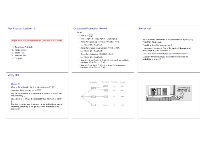
Alex Psomas: Lecture 15. Conditional Probability: Review Monty Hall Recall: ◮ Pr [ A | B ] = Pr [ A ∩ B ] Pr [ B ] . ◮ Hence, Pr [ A ∩ B ] = Pr [ B ] Pr [ A | B ] = Pr [ A ] Pr [ B | A ] . 3 closed doors. Behind one of the doors there is a prize (car). Bayes’ Rule, Mutual Independence, Collisions and Collecting ◮ A and B are positively correlated if Pr [ A | B ] > Pr [ A ] , The others have goats. i.e., if Pr [ A ∩ B ] > Pr [ A ] Pr [ B ] . You pick a door. Say door number 1 1. Conditional Probability ◮ A and B are negatively correlated if Pr [ A | B ] < Pr [ A ] , I open door 2 or door 3. One of the two that I know doesn’t 2. Independence have the prize. Say it was door 2 i.e., if Pr [ A ∩ B ] < Pr [ A ] Pr [ B ] . 3. Bayes’ Rule I ask: Would you like to change your door to number 3? ◮ A and B are independent if Pr [ A | B ] = Pr [ A ] , 4. Balls and Bins Question: What should you do in order to maximize the i.e., if Pr [ A ∩ B ] = Pr [ A ] Pr [ B ] . 5. Coupons probability of winning? ◮ Note: B ⊂ A , and Pr [ A ] � = 1, Pr [ B ] � = 0, ⇒ A and B are positively correlated. ( Pr [ A | B ] = 1 > Pr [ A ]) ◮ Note: A ∩ B = / 0 , Pr [ A ] , Pr [ B ] � = 0, ⇒ A and B are negatively correlated. ( Pr [ A | B ] = 0 < Pr [ A ]) Monty Hall Change!!!! What is the probability that the prize is in door 3? 2 3 ! How does that make any sense???? Say the original door where the prize is random. So each door has probability 1 3 . You pick door 1. What’s the probability that it’s in either 2 or 3? 2 3 The door I opened wasn’t random! I knew it didn’t have a prize!! Therefore, switching, is like getting to pick two doors at the beginning!

A B b A B B A Balls in bins Conditional Probability: Pictures Bayes and Biased Coin Illustrations: Pick a point uniformly in the unit square I throw 5 (indistinguishable) balls in two bins. What is the probability that the first bin is empty? 1 1 1 1. Approach 1: There are 6 outcomes: ( 5 , 0 ) , ( 4 , 1 ) , ( 3 , 2 ) , ( 2 , 3 ) , ( 1 , 4 ) , ( 0 , 5 ) . Probability that the first bin is empty is 1 6 2. Approach 2: I pretend I can tell the balls apart. There are 2 5 outcomes: ( 1 , 1 , 1 , 1 , 1 ) , ( 1 , 1 , 1 , 1 , 2 ) , . . . ( 2 , 2 , 2 , 2 , 2 ) . ( x , 1 , x , x , x ) means that the second ball I threw landed in 0 0 0 0 1 0 1 0 1 b 2 b 1 b 1 b 2 the first bin. Pick a point uniformly at random in the unit square. Then Probability that the first bin ie empty is 1 2 5 . The fact that I Pr [ A ] = 0 . 5 ; Pr [¯ A ] = 0 . 5 can tell them apart shouldn’t change the probability. ◮ Left: A and B are independent. Pr [ B ] = b ; Pr [ B | A ] = b . Pr [ B | A ] = 0 . 5 ; Pr [ B | ¯ A ] = 0 . 6 ; Pr [ A ∩ B ] = 0 . 5 × 0 . 5 ◮ Middle: A and B are positively correlated. Well... I guess probability is wrong... Pr [ B ] = 0 . 5 × 0 . 5 + 0 . 5 × 0 . 6 = Pr [ A ] Pr [ B | A ]+ Pr [¯ A ] Pr [ B | ¯ Pr [ B | A ] = b 1 > Pr [ B | ¯ A ] A ] = b 2 . Note: Pr [ B ] ∈ ( b 2 , b 1 ) . Or...... Could one of the approaches be wrong??? 0 . 5 × 0 . 5 Pr [ A ] Pr [ B | A ] Approach 1 is WRONG! Why did we divide by | Ω | ??? ◮ Right: A and B are negatively correlated. Pr [ A | B ] = 0 . 5 × 0 . 5 + 0 . 5 × 0 . 6 = Pr [ A ] Pr [ B | A ]+ Pr [¯ A ] Pr [ B | ¯ Pr [ B | A ] = b 1 < Pr [ B | ¯ A ] Why??????? Nooooooooooooooooooooooooo A ] = b 2 . Note: Pr [ B ] ∈ ( b 1 , b 2 ) . ≈ 0 . 46 = fraction of B that is inside A Bayes: General Case Why do you have a fever? Why do you have a fever? Our “Bayes’ Square” picture: 0 . 80 Flu 0 . 15 ≈ 0 1 Ebola Other 0 . 85 Green = Fever Using Bayes’ rule, we find 0 . 15 × 0 . 80 0 . 10 Pr [ Flu | High Fever ] = 0 . 15 × 0 . 80 + 10 − 8 × 1 + 0 . 85 × 0 . 1 ≈ 0 . 58 58% of Fever = Flu Pick a point uniformly at random in the unit square. Then ≈ 0% of Fever = Ebola 10 − 8 × 1 0 . 15 × 0 . 80 + 10 − 8 × 1 + 0 . 85 × 0 . 1 ≈ 5 × 10 − 8 42% of Fever = Other Pr [ A m ] = p m , m = 1 ,..., M Pr [ Ebola | High Fever ] = Pr [ B | A m ] = q m , m = 1 ,..., M ; Pr [ A m ∩ B ] = p m q m 0 . 85 × 0 . 1 Note that even though Pr [ Fever | Ebola ] = 1, one has Pr [ Other | High Fever ] = 0 . 15 × 0 . 80 + 10 − 8 × 1 + 0 . 85 × 0 . 1 ≈ 0 . 42 Pr [ B ] = p 1 q 1 + ··· p M q M p m q m Pr [ Ebola | Fever ] ≈ 0 . The values 0 . 58 , 5 × 10 − 8 , 0 . 42 are the posterior probabilities. Pr [ A m | B ] = = fraction of B inside A m . p 1 q 1 + ··· p M q M This example shows the importance of the prior probabilities.

B B A A A Bayes’ Rule Operations Independence Pairwise Independence Recall : Flip two fair coins. Let A and B are independent ◮ A = ‘first coin is H’ = { HT , HH } ; ⇔ Pr [ A ∩ B ] = Pr [ A ] Pr [ B ] ◮ B = ‘second coin is H’ = { TH , HH } ; ⇔ Pr [ A | B ] = Pr [ A ] . ◮ C = ‘the two coins are different’ = { TH , HT } . Consider the example below: ¯ 1 0.1 0.15 0.25 0.25 2 0.15 0.1 Bayes’ Rule is the canonical example of how information A , C are independent; B , C are independent; 3 changes our opinions. A ∩ B , C are not independent. ( Pr [ A ∩ B ∩ C ] = 0 � = Pr [ A ∩ B ] Pr [ C ] .) ( A 2 , B ) are independent: Pr [ A 2 | B ] = 0 . 5 = Pr [ A 2 ] . A did not say anything about C and B did not say anything ( A 2 , ¯ B ) are independent: Pr [ A 2 | ¯ B ] = 0 . 5 = Pr [ A 2 ] . about C , but A ∩ B said something about C ! ( A 1 , B ) are not independent: Pr [ A 1 | B ] = 0 . 1 0 . 5 = 0 . 2 � = Pr [ A 1 ] = 0 . 25. Example 2 Mutual Independence Mutual Independence Flip a fair coin 5 times. Let A n = ‘coin n is H’, for n = 1 ,..., 5. Definition Mutual Independence Theorem Then, A m , A n are independent for all m � = n . (a) The events A 1 ,..., A 5 are mutually independent if (a) If the events { A j , j ∈ J } are mutually independent and if K 1 and K 2 are disjoint finite subsets of J , then Also, Pr [ ∩ k ∈ K A k ] = Π k ∈ K Pr [ A k ] , for all K ⊆ { 1 ,..., 5 } . A 1 and A 3 ∩ A 5 are independent . ∩ k ∈ K 1 A k and ∩ k ∈ K 2 A k are independent. (b) More generally, the events { A j , j ∈ J } are mutually Indeed, independent if (b) More generally, if the K n are pairwise disjoint finite subsets Pr [ A 1 ∩ ( A 3 ∩ A 5 )] = 1 of J , then the events 8 = Pr [ A 1 ] Pr [ A 3 ∩ A 5 ] Pr [ ∩ k ∈ K A k ] = Π k ∈ K Pr [ A k ] , for all finite K ⊆ J . ∩ k ∈ K n A k are mutually independent. . Similarly, Example: Flip a fair coin forever. Let A n = ‘coin n is H.’ Then the (c) Also, the same is true if we replace some of the A k by ¯ A k . events A n are mutually independent. A 1 ∩ A 2 and A 3 ∩ A 4 ∩ A 5 are independent . This leads to a definition ....

Balls in bins Balls in bins The Calculation. One throws m balls into n > m bins. One throws m balls into n > m bins. A i = no collision when i th ball is placed in a bin. Pr [ A 1 ] = 1 Pr [ A 2 | A 1 ] = 1 − 1 n Pr [ A 3 | A 1 , A 2 ] = 1 − 2 n Pr [ A i | A i − 1 ∩···∩ A 1 ] = ( 1 − i − 1 n ) . no collision = A 1 ∩···∩ A m . Product rule: Pr [ A 1 ∩···∩ A m ] = Pr [ A 1 ] Pr [ A 2 | A 1 ] ··· Pr [ A m | A 1 ∩···∩ A m − 1 ] � 1 − 1 � � 1 − m − 1 � ⇒ Pr [ no collision ] = ··· . n n Theorem: Pr [ no collision ] ≈ exp {− m 2 2 n } , for large enough n . Approximation Balls in bins Theorem: Pr [ no collision ] ≈ exp {− m 2 2 n } , for large enough n . � � � � 1 − 1 1 − m − 1 ⇒ Pr [ no collision ] = ··· . n n Hence, m − 1 m − 1 ln ( 1 − k ( − k n ) ( ∗ ) ln ( Pr [ no collision ]) = ∑ n ) ≈ ∑ k = 1 k = 1 ( † ) ≈ − m 2 − 1 m ( m − 1 ) = n 2 2 n ( ∗ ) We used ln ( 1 − ε ) ≈ − ε for | ε | ≪ 1. ( † ) 1 + 2 + ··· + m − 1 = ( m − 1 ) m / 2. exp {− x } = 1 − x + 1 2 ! x 2 + ··· ≈ 1 − x , for | x | ≪ 1 . Hence, − x ≈ ln ( 1 − x ) for | x | ≪ 1.

Balls in bins The birthday paradox Today’s your birthday, it’s my birthday too.. Theorem: Probability that m people all have different birthdays? Pr [ no collision ] ≈ exp {− m 2 2 n } , for large enough n . With n = 365, one finds √ Pr [ collision ] ≈ 1 / 2 if m ≈ 1 . 2 365 ≈ 23 . In particular, Pr [ no collision ] ≈ 1 / 2 for m 2 / ( 2 n ) ≈ ln ( 2 ) , i.e., If m = 60, we find that √ � m ≈ 2ln ( 2 ) n ≈ 1 . 2 n . Pr [ no collision ] ≈ exp {− m 2 60 2 2 n } = exp {− 2 × 365 } ≈ 0 . 007 . √ E.g., 1 . 2 20 ≈ 5 . 4. Roughly, Pr [ collision ] ≈ 1 / 2 for m = √ n . ( e − 0 . 5 ≈ 0 . 6.) If m = 366, then Pr [ no collision ] = 0. (No approximation here!) The birthday paradox Checksums! Coupon Collector Problem. Consider a set of m files. Each file has a checksum of b bits. There are n different baseball cards. How large should b be for Pr [ share a checksum ] ≤ 10 − 3 ? (Brian Wilson, Jackie Robinson, Roger Hornsby, ...) One random baseball card in each cereal box. Claim: b ≥ 2 . 9ln ( m )+ 9. Proof: Let n = 2 b be the number of checksums. Theorem: If you buy m boxes, We know Pr [ no collision ] ≈ exp {− m 2 / ( 2 n ) } ≈ 1 − m 2 / ( 2 n ) . Hence, (a) Pr [ miss one specific item ] ≈ e − m n Pr [ no collision ] ≈ 1 − 10 − 3 ⇔ m 2 / ( 2 n ) ≈ 10 − 3 (b) Pr [ miss any one of the items ] ≤ ne − m n . ⇔ 2 n ≈ m 2 10 3 ⇔ 2 b + 1 ≈ m 2 2 10 ⇔ b + 1 ≈ 10 + 2log 2 ( m ) ≈ 10 + 2 . 9ln ( m ) . Note: log 2 ( x ) = log 2 ( e ) ln ( x ) ≈ 1 . 44ln ( x ) .