AI2 - Module 3 Task 5: Learning from Data Overview Task 5: - - PowerPoint PPT Presentation

Artificial Intelligence 2Bh

AI2 - Module 3

Task 5: Learning from Data Task 6: Coping with Incomplete Information Lecturer: Mark Steedman e-mail: steedman@inf.ed.ac.uk Office: Room 2R.14, 2 Buccleuch Place Notes: Copies of the lecture slides. Activities: 18 lectures. Two practicals covering both tasks. Required Text: Russell & Norvig, 2nd Ed., Chaps. 13-16, 18-20. Further Reading: Tom Mitchell, Machine Learning, 1997.

AI2-LFD Introduction 1-1 course overview

Task 5: Learning from Data Overview

• 1. Introduction
• 2. Learning with Decision Trees.
• 3. Learning as Search.
• 4. Neural Networks: the Perceptron, multi-layer networks,

back-propagation. Text: Chapters 18-20 of Russell & Norvig

AI2-LFD Introduction 1-2

Learning from Data

Two related tasks in applying AI techniques to any task:

• 1. Represent relevant knowledge in a computationally tractable form.
• 2. Design and implement algorithms which effectively employ that

knowledge so represented to achieve the desired processing. Learning systems actually change and/or augment the represented knowledge on the basis of experience.

AI2-LFD Introduction 1-3

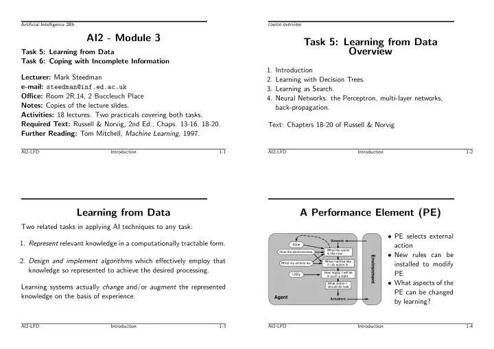
A Performance Element (PE)

Agent Environment

Sensors What it will be like if I do action A How happy I will be in such a state What action I should do now State How the world evolves What my actions do Utility Actuators What the world is like now

• PE selects external

action

• New rules can be

installed to modify PE

• What aspects of the

PE can be changed by learning?

AI2-LFD Introduction 1-4

What components of PE can change?

Examples are:

• 1. A direct mapping from conditions on the current state to actions.
• 2. A means to infer relevant properties of the world from the percept

sequence.

• 3. Information about the way the world evolves.
• 4. Information about the results of possible actions the agent can

take.

• 5. Utility information indicating the desirability of world states.

AI2-LFD Introduction 1-5

• 6. Action-value information indicating the desirability of particular

actions in particular states.

• 7. Goals that describe classes of states whose achievement maximises

the agent’s utility. Each of these components can be learned

• Have notion of performance standard

– can be hardwired: e.g. hunger, pain etc. – provides feedback on quality of agent’s behaviour

AI2-LFD Introduction 1-6

Learning from Data

We will consider a slightly constrained setup known as

Supervised Learning

• The learning agent sees a set of examples.
• Each example is labelled, i.e.

associated with some relevant information.

• The learning agent generalises by producing some representation

that can be used to predict the associated value on unseen examples.

• The predictor is used either directly or in a larger system.

AI2-LFD Introduction 1-7

A Range of Applications

Scientific research, control problems, engineering devices, game playing, natural language applications, Internet tools, commerce.

• Diagnosing diseases in plants.
• Identifying useful drugs (pharmaceutical research).
• Predicting protein folds (Genome project).
• Cataloguing space images.
• Steering a car on highway (by mapping state to action).
• An automated pilot in a restricted environment (by mapping state

to action).

AI2-LFD Introduction 1-8

• Playing Backgammon (by mapping state to its “value”).
• Performing symbolic integration (by mapping expressions to

integration operators).

• Controlling oil-gas separation.
• Generating the past tense of a verb.
• Context sensitive spelling correction (“I had a cake for desert”).
• Filtering interesting articles from newsgroups.
• Identifying interesting web-sites.
• Fraud detection (on credit card activities).
• Identifying market properties for commerce.
• Stock market prediction.

AI2-LFD Introduction 1-9

Major issues for learning problems

• What components of the performance element are to be improved.
• What

representation is used for the knowledge in those components.

• What feedback is available.
• What representation is used for the examples.
• What prior knowledge is available.

AI2-LFD Introduction 1-10

Sources and Types of Learning Systems

Is the system passive or active? Is the system taught by someone else, or must it learn for itself? Do we approach the system as a whole,

• r component by

component? Our setup of Supervised Learning implies a passive system that is taught through the selection of examples (though the “teacher” may not be helpful).

AI2-LFD Introduction 1-11

Other Types of Learning Problems

unsupervised learning The system receives no external feedback, but has some internal utility function to maximise. For example, a robot exploring a distant planet might be set to classify the forms of life it encounters there. reinforcement learning The system is trained with post-hoc evaluation of every output. For example, a system to play backgammon might be trained by letting it play some games, and at the end of each game telling it whether it won or lost. (There is no direct feedback on every action.)

AI2-LFD Introduction 1-12

Supervised Learning

• Some part of the performance element is modelled as a function

f - a mapping from possible descriptions into possible values.

• A labelled example is a pair (x, v) where x is the description and

the intention is that the v = f(x).

• The learner is given some labelled examples.
• The learner is required to find a mapping h (for hypothesis) that

can be used to compute the value of f on unseen descriptions: “h approximates f”

AI2-LFD Introduction 1-13

Supervised Learning: Example

The first major practical application of machine learning techniques was indicated by Michalski and Chilausky’s (1980) soybean experiment. They were presented with information about sick soya bean plants whose diseases had been diagnosed.

• Each plant was described by values of 35 attributes, such as

leafspots halos and leafspot size, as well as by its actual disease.

• The plants had 1 of 4 types of diseases.

AI2-LFD Introduction 1-14

• The learning system automatically inferred a set of rules which

would predict the disease of a plant on the basis of its attribute values.

• When tested with new plants, the system predicted the correct

disease 100% of the time. Rules constructed by human experts were only able to achieve 96.2%.

• However, the learned rules were much more complex than those

extracted from the human experts.

AI2-LFD Introduction 1-15

Supervised Learning with Decision Trees Overview

• 1. Attribute-Value representation of examples
• 2. Decision tree representation
• 3. Supervised learning methodology
• 4. Decision tree learning algorithm
• 5. Was learning successful ?
• 6. Some applications

Text: Sections 18.2-18.3 of Russell & Norvig

AI2-LFD Decision Trees 2-1

Supervised Learning with Decision Trees

• Some part of the performance element is modelled as a function

f - a mapping from possible descriptions into possible values.

• A labelled example is a pair (x, v) where x is the description and

the intention is that v = f(x).

• The learner is given some labelled examples.
• The learner is required to find a mapping h (for hypothesis) that

can be used to compute the value of f on unseen descriptions.

• h is represented by a decision tree.

AI2-LFD Decision Trees 2-2

Attribute-Value Representation for Examples

The mapping f decides whether a credit card be granted to an

• applicant. What are the important attributes or properties ?

Credit History What is the applicant’s credit history like? (values: good, bad, unknown) Debt How much debt does the applicant have? (values: low, high) Collateral Can the applicant put up any collateral? (values: adequate, none)

AI2-LFD Decision Trees - Representing Examples 2-3

Income How much does the applicant earn? (values: numerical) Dependents Does the applicant have any Dependents ? (values: numerical) The last two attributes are numerical. We may need to discretize them e.g. using (values: > 10000, < 10000) for Income and (values: yes, no) for Dependents.

AI2-LFD Decision Trees - Representing Examples 2-4

Example (cont.)

A set of examples (descriptions and labels) can be described as in the following table.

Example Attributes Goal Credit History Debt Collateral Income Dependents Yes/no X1 Good Low Adequate 20K 3 yes X2 Good High None 15K 2 yes X3 Good High None 7K no X4 Bad Low Adequate 15K yes X5 Bad High None 10k 4 no X6 Unknown High None 11K 1 no X7 Unknown Low None 9k 2 no X8 Unknown Low Adequate 9K 2 yes X9 Unknown Low None 19k yes

The learner is required to find a mapping h that can be used to compute the value of f on unseen descriptions.

AI2-LFD Decision Trees - Representing Examples 2-5

Example (cont.)

Here the only possible values for h are {yes, no}. Such mappings are called Boolean functions. They can be used to model concepts, where yes means that the description refers to an object that belongs to the concept. In our example the concept is “person who should be given credit”.

AI2-LFD Decision Trees - Representing Examples 2-6

Supervised Learning: Terminology

• An example describes the value of each of the attributes and

the value of the goal predicate.

• The value of the goal predicate is called the classification or the

label.

• For boolean goal predicates we identify positive examples and

negative examples: If the classification is “yes” (or TRUE) the example is positive. If the classification is “no” (or FALSE), the example is negative.

• The complete set of examples is the training set.

AI2-LFD Decision Trees 2-7

Decision Trees: Example

YES NO INCOME < 10,000 >10,000 YES NO INCOME < 10,000 >10,000 CREDIT HISTORY DEBT NO COLLATERAL UNKNOWN BAD GOOD YES YES COLLATERAL DEBT YES HIGH LOW ADEQUATE NONE LOW HIGH NO

AI2-LFD Decision Trees: the Representation 2-8

Knowledge Representation

A Decision Tree takes as input an object or situation described by a set of properties (attributes) and outputs a yes/no decision.

• Decision trees represent Boolean Functions.
• Each internal node in the tree corresponds to a test of a value of
• ne of the properties.
• Each branch of the tree is labelled with the possible value of the

test.

• Each leaf-node specifies the Boolean value to be returned if the

leaf is reached.

AI2-LFD Decision Trees: the Representation 2-9

Knowledge Representation (cont.)

• Any path through a decision tree can be represented by a

conjunction of logical tests.

• Can write an equivalent logical description of Yes leaves (or No

leaves).

• Logically, a decision tree is a collection of individual implications

corresponding to paths in tree ending in Yes nodes.

• Attributes correspond to propositions

E.g. ∀m. credit story(m, good) ∧ debt(m, low) ⇒ given credit(m)

AI2-LFD Decision Trees: the Representation 2-10 Expressive Power

Expressive Power of Decision Trees

• Despite the quantifier ∀, Decision Tree language is essentially

propositional, limited to defining a new property over a single variable in terms of a logical combination of attributes of that variable—hence a decision tree cannot represent a test such as IF credit-history(man, bad) AND income(man, < 10K) AND married-to(man, wife) AND income(wife, < 10K) THEN no credit

AI2-LFD Decision Trees: the Representation 2-11 Expressive Power

• Any Boolean Function can be written as a tree but some such

functions would require a very large tree. The obvious translation: (1) at top level split on first attribute (2) at 2nd level split on 2nd attribute . . . may produce large trees (due to exponential growth).

• NB The ideas here can be generalised for situations where there

are more than two outcomes.

AI2-LFD Decision Trees: the Representation 2-12

Supervised Learning: How?

• The learner is required to find a mapping h that can be used to

compute the value of f on unseen descriptions.

• In order to do that, machine learning programs normally try to

find a hypothesis h that gives correct classification to the training set. Is this reasonable?

AI2-LFD DTs: supervised learning methodology 2-13

Decision Tree Induction: Quality

(How to induce decision trees from examples)

• A trivial solution has one path to a leaf for each example.
• However, this just memorises the examples, and does not extract

a pattern.

• A decision tree should be able to extrapolate from the given

examples to examples it has not seen.

• A good decision tree should not only agree with the examples. It

should also be concise.

AI2-LFD DTs: supervised learning methodology 2-14

Supervised Learning: How? (cont.)

Principle of Ockham’s Razor The most likely hypothesis is the simplest one consistent with all the observations. This general argument has been given a rigorous quantitative treatment in computational learning theory. Can We Find the Smallest Decision Tree ? There is no known efficient solution to this problem! What we can do is devise heuristics that will often give us fairly small trees.

AI2-LFD DTs: supervised learning methodology 2-15

Decision Tree Learning Algorithm

• Choose a “good attribute” to put at the top level.
• Take this attribute and split up the examples into subsets, one

for each value of the chosen attribute.

• For each subset that has only positive or only negative examples,

attach a leaf with the corresponding value.

• Each subset that has both positive and negative examples, needs

a new decision tree. ⇒ Apply the decision-tree-learning-algorithm recursively. NB recursion has fewer examples and one fewer attribute

AI2-LFD Decision Trees: Learning Algorithm 2-16

Applying the Algorithm: Example

Choose Collateral: Value Adequate induces subset: {X1,X4,X8} Value None induces subset: {X2,X3,X5,X6,X7,X9} {X1,X4,X8} all labelled yes - attach a leaf to this branch. {X2,X3,X5,X6,X7,X9} has both positive and negative examples. Choose Income: Value < 10K induces subset: {X3,X7} Value ≥ 10K induces subset: {X2,X5,X6,X9} {X3,X7} all labelled no - attach a leaf to this branch.

AI2-LFD Decision Trees: Learning Algorithm 2-17

{X2,X5,X6,X9} has both positive and negative examples. Choose Debt: Value Low induces subset: {X9} - attach a leaf to it Value High induces subset: {X2,X5,X6} {X2,X5,X6} has both positive and negative examples. Choose Credit History: Value Good induces subset: {X2} - attach a leaf to it Value Bad induces subset: {X5} - attach a leaf to it Value Unknown induces subset: {X6} - attach a leaf to it

AI2-LFD Decision Trees: Learning Algorithm 2-18

A Better Decision Tree

NO BAD COLLATERAL YES GOOD INCOME LOW HIGH DEBT LOW HIGH CREDIT HISTORY UNKNOWN GOOD BAD NO NO YES YES

• This is a better tree than Slide 2-8, with fewer nodes including

leaf nodes

• Neither tree needs to use the Dependents property

AI2-LFD Decision Trees: Learning Algorithm 2-19

What if . . .

• If a value induces an empty subset {}, no such example has

been observed: ⇒ return a default value using the majority classification of the parent set.

• If there are no attributes left, but still positive and negative

examples, then there is a problem! The algorithm returns the majority classification of the remaining examples.

AI2-LFD Decision Trees: Learning Algorithm 2-20

Noisy Training Set

If there are no attributes left, but still positive and negative examples, then there is no decision tree that gives a correct classification to all the examples in the training set. What can be the reason?

• Some of the data may be incorrect—the data is said to be noisy.
• The attributes may not give enough information to fully describe

the situation.

• The domain may be truly non-deterministic.

Algorithm returns the majority classification of remaining examples.

AI2-LFD Decision Trees: Learning Algorithm 2-21

function DECISION-TREE-LEARNING(examples,attributes, default) returns a decision tree inputs: examples, set of examples attributes, set of attributes default, default value for the goal predicate if examples is empty then return default else if all examples have the same classification then return the classification else if attributes is empty then return MAJORITY-VALUE(examples) else best

• CHOOSE-ATTRIBUTE(attributes, examples)

tree

• a new decision tree with root test best

for each value vi of best do examplesi

• ✁

elements of examples with best = vi

subtree

• DECISION-TREE-LEARNING(examplesi, attributes

best, MAJORITY-VALUE(examples)) add a branch to tree with label vi and subtree subtree end return tree

AI2-LFD Decision Trees: Learning Algorithm 2-22

• T. Mitchell, Machine Learning, Sec. 3.7.1

Noise and Overfitting

Noisy examples can also lead to growing the tree too much (so as to classify noisy examples correctly). Often, using a smaller part of the tree is better. How can we avoid overfitting ?

• Stop growing when data split not statistically significant

(small number of examples). or

• Grow full tree, then post-prune.

AI2-LFD Decision Trees: Learning Algorithm 2-23

Effect of Overfitting

0.5 0.55 0.6 0.65 0.7 0.75 0.8 0.85 0.9 10 20 30 40 50 60 70 80 90 100 Accuracy Size of tree (number of nodes) On training data On test data

AI2-LFD Decision Trees: Learning Algorithm 2-24

Choosing attributes

Imagine we have 100 positive and 100 negative examples. Use notation [100P, 100N] to describe this. Imagine we have 3 attributes generating the following splits:

• A1 generates [100P, 0N], [0P, 100N].
• A2 generates [70P, 30N], [30P, 70N].
• A3 generates [50P, 50N], [50P, 50N].

Which attribute is the best one? and the worst?

AI2-LFD Decision Trees: Learning Algorithm 2-25

Choosing attributes

Credit History is NOT a good attribute to start with.

UNKNOWN GOOD BAD +

• X1 X2

X3 X4 X5 +

• +

_ X8 X9 X6 X7 + X1 X2 X4 X8 X9

• X3 X5 X6 X7

CREDIT HISTORY

Has three possible outcomes, each of which has both +ve and -ve examples

AI2-LFD Decision Trees: Learning Algorithm 2-26

Choosing attributes

Collateral gives a definite response (Yes) for 3 cases.

ADEQUATE NONE + X1 X4 X8

• + X2 X9
• X3 X5 X6 X7

+ X1 X2 X4 X8 X9

• X3 X5 X6 X7

COLLATERAL

AI2-LFD Decision Trees: Learning Algorithm 2-27

Revision: Information Content

The information content (IC) of an event is the amount of new information communicated when we learn about the event. The information content of the event X = i, where X is a random variable and i is the outcome, is defined as IC(X = i) = log2 1 p(X = i). The definition agrees with a number of common-sense ideas regarding ‘information’:

AI2-LFD Decision Trees: Learning Algorithm 2-28

Revision: Information Content

• 1. More surprising events provide more information.

For example, if X is a random variable representing the current weather in Edinburgh, the information content of the event ‘sunny’, p(sunny = 0.001), IC = 11 bits, is higher than that of the event ‘cloudy’, p(cloudy = 0.8), IC = 0.322 bits.

• 2. Learning that an event that was bound to happen, did happen,

provides no information. Such an event has a probability 1. Since log2 1 = 0, IC = 0 bits.

AI2-LFD Decision Trees: Learning Algorithm 2-29

Revision: Information Content

• 1. Learning the outcome of related random variables reduces the

information content. For example, the information provided by learning that a randomly selected English character is ‘u’ is lower when we already know that the previous letter was‘q’.

AI2-LFD Decision Trees: Learning Algorithm 2-30

Revision: Entropy

The entropy of a random variable, I(X), is an average of the information content over the outcomes of the random variable. If a variable X has N possible outcomes, I(X) =

N

• i=1

p(X = i) log2 1 p(X = i). Entropy can be thought of as the average uncertainty of the random

• variable. Prediction is easier when the entropy is lower since we are

less uncertain (on average).

AI2-LFD Decision Trees: Learning Algorithm 2-31

Revision: Entropy

For example, the entropy of a coin is maximized when it is fair i.e. when p(heads = 0.5) and p(tail = 0.5), I(X) = 0.5 · log2

1 0.5 + 0.5 · log2 1 0.5 = log2 2 = 1 bit. A fair coin is also most

difficult to predict. When the coin is biased, say, p(heads = 0.8) and p(tails = 0.2), the entropy will be lower i.e. 0.8 · log2

1 0.8 + 0.2 · log2 1 0.2 = 0.722

bits, and we can win money if we predict heads...

AI2-LFD Decision Trees: Learning Algorithm 2-32

Revision: Entropy

Decision trees predict a class variable by asking questions about (hopefully correlated) attributes of an input example. The answers to these questions reduce the entropy (uncertainty) of the class assignment making prediction gradually easier at each node in the tree.

AI2-LFD Decision Trees: Learning Algorithm 2-33

Choosing attributes - the Details

The current example set has p positive and n negative examples. A split on attribute A with v values generates v subsets with pi, ni examples respectively (i = 1 . . . v). I(p, n) = p p + n log(p + n p ) + n p + n log(p + n n ) measures the entropy of the current set. Trying to measure how far we are from having a single label. I(X, X) = 1 and I(0, X) = I(X, 0) = 0 for any value of X

AI2-LFD Decision Trees: Learning Algorithm 2-34

Remainder(A) =

v

• i=1

pi + ni p + n I(pi, ni) where A is an attribute, measures average entropy after split. Again, trying to measure how far we are from having a single label. Gain(A) = I(p, n) − Remainder(A) tries to measure the improvement obtained by the split. Gain(Collateral) = I(5, 4) − (6

9I(2, 4) + 3 9I(3, 0)) = 5 9 log 9 5 + 4 9 log 9 4 − 6 9 · 2 6 log 6 2 − 6 9 · 4 6 log 6 4 − 3 9 · 3 3 log 3 3 − 3 9 · 0 3 log 3 0 = 0.38 AI2-LFD Decision Trees: Learning Algorithm 2-35

Choosing attributes - the Details

• 1. For each attribute A compute Gain(A)
• 2. Choose the attribute that has the maximum Gain(A)

This is only a heuristic. But it works well in practice. Other criteria for choosing attributes were developed (including dealing with numerical attributes directly).

AI2-LFD Decision Trees: Learning Algorithm 2-36

Decision Tree Quality

Having used a heuristic for finding a small decision tree, our hope was that this tree can be used to (correctly) compute the value of f on unseen instances.

• What if this tree is consistent with the training set but far from

correct otherwise?

• Can we assess the quality of the tree?

Some answers are provided by statistical analysis. One approach, plotting learning curves, also gives some qualitative impression.

AI2-LFD Decision Trees: Assessment 2-37

Assessing decision trees

• 1. Collect a large set of examples.
• 2. Divide into two disjoint sets: the training set and the test set.
• 3. Use the learning algorithm with the training set to generate a

hypothesis H.

• 4. Measure the percentage of examples in the test set, correctly

classified by H.

• 5. Repeat steps 1-4 with different sizes of training sets, and different

randomly selected training sets of each size.

• 6. Plot the training set size against the average % correct on test

sets —this is called the learning curve.

AI2-LFD Decision Trees: Assessment 2-38

1 0.4 % correct on test set Training set size 100 50

AI2-LFD Decision Trees: Assessment 2-39

Designing Oil Platform Equipment

• In 1986, BP used an expert system called GASOIL for designing
• il-gas separation systems for offshore platforms.
• Separations are done by a system whose design depends on a large

number of attributes—relative proportions of oil, gas, water, flow- rate, pressure, density, viscosity, temperature....

• GASOIL system contained 2500 rules!
• Building such a system by hand would have taken 10 person-years.
• Using decision-tree learning methods, the system was developed

in 100 person days.

AI2-LFD Decision Trees: Applications 2-40

Learning To Fly

• An automated controller can be constructed by learning the

correct mapping from a state of the system to the correct action.

• Sammut et al. 1992 used this method for learning to fly a Cessna
• n a flight simulator, in a restricted environment.
• Data generated by watching human pilots perform a flight plan

30 times, each action taken resulted in a training examples being created.

AI2-LFD Decision Trees: Applications 2-41

• 90,000 examples were obtained, each described by 20 state values,

and a resulting action.

• Decision tree created and converted into C code for use by the

flight simulator (in a controlled manner).

• The program learns to fly, and at times flies better than its

teachers.

AI2-LFD Decision Trees: Applications 2-42

Sky Image Cataloguing and Analysis

System called SkyCat by (Fayad, Djorgovski, Weir, 1996).

• Task: catalogue entries for objects in images.
• Large amounts of data collected by astronomers; objects too

“faint” need special methods.

• Images split to smaller parts; various features measured on each

to generate examples.

• Relatively small number of examples classified by astronomers.
• Decision Tree methods used to learn classifiers.
• Performance:

94.1% correct on test data; results used by astronomers.

AI2-LFD Decision Trees: Applications 2-43

Learning as Search Overview

• 1. Learning can be done by searching for a good hypothesis
• 2. Learning Logical Descriptions
• 3. Current-Best-Search Learning
• 4. Version Space Learning

Text: Section 19.1 of Russell & Norvig

AI2-LFD Learning as Search 3-1 Artificial Intelligence 2Bh

Supervised Learning

The Task: The learner is required to find a mapping h that can be used to compute the value of f on unseen descriptions. The Approach: By Ockham’s Razor, the learner tries to find a concise representation for h that is consistent with all the examples. Hypothesis Space: A representation language for the possible hypotheses must be fixed. Bias: Criteria for choosing between different hypotheses (such as conciseness) are employed; this shows an a-priori bias of the learner to prefer some hypotheses to others.

AI2-LFD Learning as Search 3-2

Learning as Search

Once the hypothesis space and preference criteria are fixed this approach to learning can be viewed as a kind of search among a set of candidate concepts, the hypothesis space. This is useful since we can apply our general knowledge on search strategies to learning problems!

AI2-LFD Learning as Search 3-3

Learning Logical Descriptions: Example

Task: For instance, we could seek a definition of when it is worth waiting at a restaurant. Language: Logical expressions in the form of disjunctions of conjunctions, with negation only applying to individual predicates and with quantification only universal and over one variable. Vocabulary: Unary predicates, corresponding to Boolean properties

• f a situation, e.g. Hungry(r), Fri/Sat(r).

Binary predicates, corresponding to

• ther

attributes, e.g. Patrons(r, Full), Type(r, French). The goal predicate WillWait(r).

AI2-LFD Learning as Search: logical descriptions 3-4

Some possible hypotheses

h1 = ∀r.WillWait(r) ⇔ Patrons(r, Some) ∨ Patrons(r, Full) ∧ ¬Hungry(r) ∧ Type(r, French) ∨ Patrons(r, Full) ∧ ¬Hungry(r) ∧ Type(r, Burger) h2 = ∀r.WillWait(r) ⇔ Patrons(r, Some) ∧ Hungry(r) ∨ Patrons(r, Full) ∧ ¬Hungry(r) ∧ Type(r, French)

Note that h2 is more restrictive than h1.

AI2-LFD Learning as Search: logical descriptions 3-5

Examples

• Examples are again descriptions of objects.

The label indicates whether the goal predicate holds for the object.

• An object is described using a logical expression that has one

“free” argument, referring to the object (like decision tree examples).

• Normally, a subset of the language used for hypotheses is used

for examples. Here we do not allow disjunctions. The example X1 may be described using:

Patrons(X1, Some) ∧ Hungry(X1) ∧ Type(X1, Thai) ∧ . . .

and the classification WillWait(X1).

AI2-LFD Learning as Search: logical descriptions 3-6

Consistency

Consistency

When is an example consistent with a hypothesis? Except in the two cases: False positive: If WillWait(X1) follows from the hypothesis but X1 in fact is a negative example. Eg: Example: Patrons(X1, Some) ∧ Hungry(X1) ∧ . . . Classification: ¬WillWait(X1) Hypothesis: ∀r.WillWait(r) ⇔ Hungry(r)

AI2-LFD Learning as Search: logical descriptions 3-7 Consistency

False negative: If ¬WillWait(X2) follows from the hypothesis but X2 in fact is a positive example. Eg: Example: Patrons(X2, Full) ∧ ¬Hungry(X2) ∧ . . . Classification: WillWait(X2) Hypothesis: ∀r.WillWait(r) ⇔ Hungry(r)

AI2-LFD Learning as Search: logical descriptions 3-8

Dealing with inconsistent examples

(a) (b) (c) (d) (e) + + + + + + + − − − − − − − − − − − + + + + + + + − − − − − − − − − − − + + + + + + + + − − − − − − − − − − − + + + + + + + + − − − − − − − − − − + − + + + + + + + − − − − − − − − − − + − − −

Coping with a false negative (b) requires generalisation (c). Coping with a false positive (d) requires specialisation (e). A learning algorithm results by performing a search over the hypothesis space using generalisation and specialisation operators.

AI2-LFD Learning as Search: current best learning 3-9

Current Best Learning Algorithm

The algorithm needs to choose generalisations and specialisations (there may be several). If it gets into trouble, it has to backtrack to an earlier decision or otherwise it fails.

AI2-LFD Learning as Search: current best learning 3-10

Generalising a Description

• Remove a conjunct, e.g.

change [Hungry(r) ∧ Patrons(r, Full)] to [Hungry(r)]

• Add a disjunct, e.g.

change [Hungry(r)] to [Hungry(r) ∨ Patrons(r, Full)]

• Replace a predicate/value by a more general one, e.g.

change [Type(r, French)] to [Type(r, European)] Here we assumed that the learner knows the semantics of French and European.

AI2-LFD Learning as Search: current best learning 3-11

Specialising a Description

• Add a conjunct. e.g.

change [Hungry(r)] to [Hungry(r) ∧ Patrons(r, Full)]

• Remove a disjunct, e.g.

change [Hungry(r) ∨ Patrons(r, Full)] to [Hungry(r)]

• Replace a predicate/value by a more specific one, e.g. change

[Hungry(r)] to [V eryHungry(r)] Here we assumed that the learner knows the semantics of Hungry() and V eryHungry().

AI2-LFD Learning as Search: current best learning 3-12

CBL Example

Current Hypothesis Example Action ∀r.WillWait(r) ⇔ false X1 false negative Add disjunct ∀r.WillWait(r) ⇔ Alternate(r) X2 false positive Add conjunct ∀r.WillWait(r) ⇔ [Alternate(r) ∧ Patrons(r, Some)] X3 false negative Remove conjunct ∀r.WillWait(r) ⇔ Patrons(r, Some) X4 false negative Add disjunct ∀r.WillWait(r) ⇔ [Patrons(r, Some) ∨ (Patrons(r, Full) ∧ Fri/Sat(r))]

There were, of course, many other possibilities.

AI2-LFD Learning as Search: current best learning 3-13

Problems with CBL

Although CURRENT-BEST-LEARNING has been popular, it has a number of problems:

• It needs to store all encountered examples (to check that changes

are consistent with all of them).

• Checking over all encountered examples when a change is made

is expensive.

• It is difficult to find good heuristics.

Real hypothesis spaces are large or infinite. Backtracking may not quickly reconsider the right decision and so may take a long time.

AI2-LFD Learning as Search: current best learning 3-14

Least Commitment Search

• LCS Avoids making arbitrary decisions that might end up wrong.
• The set of hypotheses consistent with the examples seen so far is

called the version space.

• The algorithm works by successively eliminating inconsistent

hypotheses from the version space. Hence called the candidate elimination algorithm.

AI2-LFD Learning as Search: version spaces 3-15

Candidate Elimination Algorithm

(Version Space Learning)

function VERSION-SPACE-LEARNING(examples) returns a version space local variables: V, the version space: the set of all hypotheses V

• the set of all hypotheses

for each example e in examples do if V is not empty then V

• VERSION-SPACE-UPDATE(V,e)

end return V function VERSION-SPACE-UPDATE(V,e) returns an updated version space V

• ✁

h

V : h is consistent with e

AI2-LFD Learning as Search: version spaces 3-16

Compact Representation of Version Spaces

Imagine you had to represent all the numbers between 1 and 2. You could represent this set just by specifying the boundaries [1,2]. This works because numbers are ordered. Hypotheses are also ordered, in terms of specificity. For instance, for hypotheses given on Slide 3-5, h1 is more general (less specific) than h2. Representation of a version space in terms of its boundaries uses two sets: S (most specific) and G (most general).

AI2-LFD Learning as Search: version spaces 3-17 Boundary Representation

this region all inconsistent This region all inconsistent

More general More specific S 1 G1 S 2 G2 G3 . . . G

m

. . . S

n

AI2-LFD Learning as Search: version spaces 3-18

Updating the Version Space

Given the current version space (constructed from examples seen so far) and a new example, the sets S and G are updated to construct the new version space. Four cases arise:

• 1. False negative for Si: ⇒ Further generalise Si.
• 2. False positive for Si: ⇒ Remove Si from the S set.
• 3. False positive for Gj: ⇒ Further specialise Gj.
• 4. False negative for Gj: ⇒ Remove Gj from the G set.

We initialize the version space as S0 = {false}, G0 = {true}

AI2-LFD Learning as Search: version spaces 3-19

VS Example

• Possible examples: a1, a2, a3, a4, a5.

NB in order to simplify the description we are not giving the representation of examples here but just their names.

• All “good” hypotheses are marked as

nodes on the graph.

• Each hypothesis description shows the

examples that are positive for it.

• Edges

represent generalisations and specialisations.

True a2a3a4 False a1a3 a3a4 a1a5 a1 a2 a3 a4 a5

AI2-LFD Learning as Search: version spaces 3-20

VS Example

S G Example false true a5 negative false a1a3,a2a3a4 a1 negative false a2a3a4 a4 positive a4 a2a3a4 a2 negative a4 a3a4 a3 positive a3a4 a3a4 CONVERGENCE

True a2a3a4 False a1a3 a3a4 a1a5 a1 a2 a3 a4 a5

AI2-LFD Learning as Search: version spaces 3-21 Version Space

Termination

Learning with version spaces can terminate in three ways:

• 1. We get to a single concept in the version space.

⇒ Return that as the answer.

• 2. The version space becomes empty, indicating that no hypotheses

(in the given space) are consistent with all the examples. ⇒ version space “collapses”

AI2-LFD Learning as Search: version spaces 3-22

Version Space

• 3. We run out of examples, still with multiple elements in the

version space. Not clear how to classify new examples. Several possibilities: (a) Select an element of the version space at random and use it. (b) Take the majority vote of all elements in the version space. (c) When classifying a new object, allow “maybe” as well as “yes”

• r “no” (in case not all hypotheses agree).

We must be able to perform this efficiently.

AI2-LFD Learning as Search: version spaces 3-23

Version Space Learning

+ Is a complete search method (unlike heuristic methods for DTs). + Is an incremental method (no need to see all examples at once). + Has been shown by Gunter et al. (1997 AIJ) to be closely related to Assumption-Based Truth Maintenance (ATM) − Is not tolerant to noise (version space will collapse). − Will not work if arbitrary disjunctions are allowed in the concept language (generalisation then simply remembers the positive examples by rote). − May not be efficient if the sets S and G are large.

AI2-LFD Learning as Search: version spaces 3-24

Neural Networks — Overview

• 1. Overview, real neurons, basic neural computing units
• 2. Neural Networks as a Representation
• 3. Perceptrons and their learning algorithm
• 4. Useful mathematical concepts (gradient descent)
• 5. Multi-layer Perceptrons, back-propagation
• 6. Some Applications

Text: sections 20.5 of Russell & Norvig

AI2-LFD Neural Networks 4-1

Real neurons

The fundamental unit of all nervous system tissue is the neuron

Axon Cell body or Soma Nucleus Dendrite Synapses Axonal arborization Axon from another cell Synapse

AI2-LFD Neural Networks: introduction 4-2

A neuron consists of

• a soma, the cell body, which contains the cell nucleus
• dendrites: input fibres which branch out from the cell body
• an axon: a single long (output) fibre which branches out over a

distance that can vary between 1cm and 1m

• synapse: a connecting junction between the axon and other cells

AI2-LFD Neural Networks: introduction 4-3

Real Neurons - Properties

• Each neuron can form synapses with anywhere between 10 and

105 other neurons

• Signals are propagated at the synapse through the release of

chemical transmitters which raise or lower the electrical potential

• f the cell
• When the potential reaches a threshold value, an action

potential is sent down the axon

• This eventually reaches the synapses and causes potentiation of

the subsequent neurons

AI2-LFD Neural Networks: introduction 4-4

• Synapses can be inhibitory (lower the post-synaptic potential) or

excitatory (raise the post-synaptic potential)

• Synapses can also exhibit long term changes of strength in

response to the pattern of stimulation

AI2-LFD Neural Networks: introduction 4-5

Artificial Neural Networks

• A neural network is composed of a number of units connected

together by links. Each link has an associated numeric weight

• Input and output units are connected to the environment
• Weights are the long term storage, learning involves changing the

weights

• Learning modifies the weights so as to try to make the output

value(s) correct given the input values.

AI2-LFD Neural Networks: introduction 4-6

Recurrent networks allow cycles

• n

directed graph i.e. links can form arbitrary topologies. We will concentrate

• n

acyclic networks, known as feed-forward networks.

• links are unidirectional
• network computes a function
• f

the input values that depends on the weight settings

• no internal state other than

weights themselves hidden units input units

• utput

unit

AI2-LFD Neural Networks: introduction 4-7

The formal neuron

• Each unit has input links from other neurons, and a current

activation level.

• Each

unit updates its activation (output) using a local computation based on its inputs without any need for global control over the set of units as a whole.

• This formal model is a gross simplification of the detailed function
• f a neuron.

AI2-LFD Neural Networks: introduction 4-8

The formal neuron

Output g

Input Links Output Links

ini

Σ

a = g(in )

i i

aj Wj,i

Activation Function Input Function i

a

• The neuron computes the total weighted input to the neuron

ini =

• j

Wj,iaj = Wi · a

AI2-LFD Neural Networks: introduction 4-9

• Wj,i is weight on link from neuron j to neuron i, Wi is the vector
• f weights leading into unit i, and a is the vector of input values.
• computing ini is a linear operation
• A

non-linear component called the activation function g transforms the sum of weighted inputs into the final output value ai ai ← g(ini) = g(Wi · a) Note: operation in Wi · a is vector dot product

• We can use different mathematical functions for g
• Usually, all units (neurons) in network have the same activation

function

AI2-LFD Neural Networks: introduction 4-10

Activation Functions

(a) Step function (b) Sign function +1

ai

−1

ini

+1

ai ini t

(c) Sigmoid function +1

ai ini

stept(z) = if z < t 1 if z ≥ t

The step and sign functions are examples of the threshold activation function.

AI2-LFD Neural Networks: introduction 4-11

Thresholds

• For a step or sign function, with threshold value t: if ini ≥ t the

unit fires. The threshold thus corresponds to the minimum total weighted input necessary to cause the neuron to fire.

• Convenient to replace the threshold with an extra weight W0, the

bias weight, from unit 0 which always has activation a0 = −1. Since ini ≥ t ⇔ ini − t ≥ 0 ai = stept  

n

• j=1

Wj,iaj   = step0  

n

• j=0

Wj,iaj  

AI2-LFD Neural Networks: introduction 4-12 a a a

1 2 3

w w w

1 2 3

a a a

1 2 3

w w w

1 2 3

w0

• 1

threshold = w threshold = 0

4 4

a a

• Trick also useful for other activation functions, e.g. the sigmoid
• This makes the learning algorithm simpler as only weights need

to be adjusted rather than weights and threshold

AI2-LFD Neural Networks: introduction 4-13

Alternative Representation of Formal Neuron

This leads to a modified mathematical model of the formal neuron where the bias weight W0,i is connected to a fixed input a0 = −1:

Output

Σ

Input Links Activation Function Input Function Output Links

a0 = −1 ai = g(ini) ai g ini Wj,i W0,i

Bias Weight

aj

AI2-LFD Neural Networks: introduction 4-14

The Perceptron

A perceptron is a single-layer feed-forward neural network. Consider an example in which the activation function is a step function:

• Set I0 = −1
• Unit fires when

n

j=0 WjIj = n j=1 WjIj − W0 ≥ 0

• W0 is the threshold:

the unit fires when

n

j=1 WjIj ≥ W0

. .

I I I

• 1

1 2 n

Σ

W W W W

n 1 2

threshold in = Σ W I

j j

AI2-LFD Neural Networks: representation 4-15

Computing Boolean Functions with Perceptrons

AND

W0 = 1.5 W1 = 1 W2 = 1

OR

W2 = 1 W1 = 1 W0 = 0.5

NOT

W1 = –1 W0 = – 0.5

Units with a (step) threshold activation function can act as logic gates, given appropriate input and bias weights.

AI2-LFD Neural Networks: representation 4-16

AND-gate truth table Bias input

• utput

a0 a1 a2

• 1
• 1

1

• 1

1

• 1

1 1 1 AND = step1.5(1 · a1 + 1 · a2) = step0(1.5 · −1 + 1 · a1 + 1 · a2) However, single-layer feed-forward nets (i.e. perceptrons) cannot represent all Boolean functions

AI2-LFD Neural Networks: representation 4-17

Some Geometry

• In 2 dimensions w1x1 +w2x2 −w0 = 0 defines a line in the plane.
• In higher dimensions n

i=1 wixi − w0 = 0 defines a hyperplane.

• The decision boundary of a perceptron is a hyperplane.
• If a hyperplane can separate all outputs of one type from outputs
• f the other type, the problem is said to be linearly separable.

AI2-LFD Neural Networks: representation 4-18

XOR is not linearly separable

I1 I2 XOR(I1, I2) (a) (b) 1 1 (c) 1 1 (d) 1 1

• Function as 2-dimensional plot based on values of 2 inputs
• black dot: XOR(I1, I2) = 1 and white dot: XOR(I1, I2) = 0
• Cannot draw a line that separates black dots from white ones

AI2-LFD Neural Networks: representation 4-19

Multilayer Neural Network

Can represent XOR using a network with two inputs, a hidden layer of two units, and

• ne
• utput.

A step (threshold) activation function is used at each unit (threshold weights (not shown) are all zero). Many architectures possible, this is an AND- NOT OR AND-NOT network.

1 1 −1 −1 1 1

In fact, any Boolean function can be represented, and any bounded continuous function can be approximated.

AI2-LFD Neural Networks: representation 4-20

Single Layer — Multiple Outputs

• Each output unit is independent
• f the others; each weight only

affects one output unit.

• We can limit our study to single-
• utput Perceptrons.
• Use several of them to make a

multi-output perceptron.

Perceptron Network Single Perceptron Input Units Units Output Input Units Unit Output

O Ij Wj,i Oi Ij Wj

AI2-LFD Neural Networks: representation 4-21

Supervised Learning: How?

• The learner sees labelled examples e = (Ie, Te)

such that f(Ie) = Te.

• The learner is required to find a mapping h that can be used to

compute the value of f on unseen descriptions.

• In order to do that, machine learning programs normally try to

find a hypothesis h that gives correct classification to the training set (or otherwise minimises the number of errors).

AI2-LFD Neural Networks: learning Perceptrons 4-22

Learning Perceptrons — Basic Idea

• Important Note: We assume a threshold activation function,

namely a step function, in the next few slides.

• Start by assigning arbitrary weights to W.
• On each example e = (I, T):

classify e with current network: O ← step0(W · I) = step0( WiIi) if O = T (correct prediction) do nothing. if O = T change W “in the right direction”. But what is “the right direction” ?

AI2-LFD Neural Networks: learning Perceptrons 4-23 The Right Direction

• if T = 1 and O = 0 we want to increase W · I = WiIi

Can do this by assigning Wnew = W + ηI since Wnew · I = W new

i

Ii = WiIi + η IiIi > WiIi

• Amount of increase controlled by parameter 0 < η < 1
• if T = 0 and O = 1 we want to decrease W · I = WiIi

Can do this by assigning Wnew = W − ηI since Wnew · I = W new

i

Ii = WiIi − η IiIi < WiIi

• In both cases we can assign Wnew = W + ηI(T − O)

AI2-LFD Neural Networks: learning Perceptrons 4-24 Perceptron Learning Algorithm (Version 1)

function perceptron-learning(examples) returns a perceptron hyp. network ← a network with randomly assigned weights repeat for each e in examples do O ← perceptron-output(network,Ie) T ← required output for Ie update weights in network based on Ie, O and T W ← W + η Ie (T − O) end until all examples correctly predicted or other stopping criterion return NEURAL-NET-HYPOTHESIS(network) Perceptron algorithm with step (threshold) activation function.

AI2-LFD Neural Networks: learning Perceptrons 4-25

Perceptron Learning Algorithm

• 0 < η < 1 is known as the learning rate, other symbols e.g. α, ǫ

used by different authors

• Rosenblatt (1960) showed that the PLA converges to W that

classifies the examples correctly (if this is possible).

• PLA behaves well with noisy examples.
• Note that PLA given above is an incremental algorithm; batch

version also possible.

AI2-LFD Neural Networks: learning Perceptrons 4-26

PLA:Example

• Assume

that

• utput

O=1, and target is T=0, ⇒ T-O=-1

• W0 ← W0 + η ∗ (−1) ∗ (−1)
• W1 ← W1 + η ∗ I1 ∗ (−1)
• W2 ← W2 + η ∗ I2 ∗ (−1)
• 1

I I O

2 1

AI2-LFD Neural Networks: learning Perceptrons 4-27

Understanding the PLA

• Will look at a simpler problem: learning a linear model

y = W · I = WiIi.

• For example: y = w0 + w1x

the model has unknown parameters w0, w1.

• We want to determine these on the basis of some training data.
• We can then use the model to generalize, i.e. to predict outputs

for new inputs.

• Trivial without noise but not so with noise.

AI2-LFD Neural Networks: gradient descent 4-28

Weight space

• Any linear model has a particular

number of weights (parameters).

• Particular

values for these parameters can be thought of as a point in weight space.

• Can

measure the cumulative error as function of parameters.

1 2

• 1
• 2
• 1
• 2

2 1 w w

1

AI2-LFD Neural Networks: gradient descent 4-29

Error Function

• Use an error function, E = 1

2

• e(Te − Oe)2
• Has desirable property that E = 0 if Te = Oe for all e.
• So, E = 0 can be obtained if there is no noise.
• Otherwise E > 0 but we can try to minimise it.
• Each value of W generates a value of E, call it E(W).

We are looking for W that minimises E(W).

AI2-LFD Neural Networks: gradient descent 4-30

Error Function — Example

• Fit y = w0 + w1x with 3 examples (the form is (x, y)):

(1, 9), (2, 7), (3, 4).

• Error is

E(W) =1 2

• (9 − w1 − w0)2 + (7 − 2w1 − w0)2 + (4 − 3w1 − w0)2

=1.5w2

0 + 7w2 1 − 20w0 − 35w1 + 6w0w1 + 73 AI2-LFD Neural Networks: gradient descent 4-31

Error Surface

• “Best” model corresponds to the the

lowest point on the error surface.

• Our problem has a single minimum

(can be obtained analytically).

• General, non-linear problems, have

a difficulty with local minima.

• ⇒ Search using methods that “go

downhill” on the error surface.

E w w B C . A .

2 1

grad(E)

AI2-LFD Neural Networks: gradient descent 4-32

Gradient descent

• If E(W) is the error function, then the derivative

∂E ∂Wi measures

the slope of the error surface in the Wi direction.

• This is summarised in vector notation as:

g = ∂E

∂W =

  

∂E ∂W0

. . .

∂E ∂Wn

  

• Locally, if we are at point W, the quickest way to decrease E is

to take a step in the direction −g.

• Given a formula for E,

∂E ∂Wi

can often be derived with straightforward algebra.

AI2-LFD Neural Networks: gradient descent 4-33

Gradient Descent Algorithm

Initialize W while E(W) is unacceptably high calculate g = ∂E

∂W

W ← W − ηg end while return W As in the PLA η is the learning rate. Here updates are in batch (error computed on all examples); incremental version as in PLA also possible.

AI2-LFD Neural Networks: gradient descent 4-34

Example (continued)

• Fit y = w0 + w1x with 3 examples (the form is (x, y)):

(1, 9), (2, 7), (3, 4).

• Error is E(W) = 1.5w2

0 + 7w2 1 − 20w0 − 35w1 + 6w0w1 + 73

• Partial derivatives:

∂E ∂w0 = 3w0 − 20 + 6w1 ∂E ∂w1 = 14w1 − 35 + 6w0

• Initial guess: w0 = 0, w1 = 0; η = 0.1

AI2-LFD Neural Networks: gradient descent 4-35

• Iteration:

w0 ← w0 − 0.1(3w0 − 20 + 6w1) w1 ← w1 − 0.1(14w1 − 35 + 6w0)

• w0 ← −0.1 · −20 = 2; w1 ← −0.1 · −35 = 3.5
• w0 ← 2 − 0.1(6 − 20 + 21) = 1.3

w1 ← 3.5 − 0.1(49 − 35 + 12) = 0.9

• . . .
• Convergence w0 = 11.66; w1 = −2.50

changes to weights < 10−4 after 226 iterations

AI2-LFD Neural Networks: gradient descent 4-36

Linear Models Again

• O = W · I = WiIi
• Use an error function, E = 1

2

• e(Te − Oe)2
• ∂E

∂Wi = −(Te − Oe)∂Oe ∂Wi = −(Te − Oe)Ii

• So the update is: Wi ← Wi + η(Te − Oe)Ii.
• PLA uses the same update!

The formula however does not correspond to its O function (the derivative of step is not very useful). NB This just says that it does not correspond to our analysis not that it is a bad algorithm.

AI2-LFD Neural Networks: gradient descent 4-37

Problems with Gradient Descent

• Need to choose η (Too small ⇒ too slow; Too big, unstable).
• Local minima.
• Plateaux.
• Gradient descent is a “hill-climbing” (actually “hill-descending”)

search: An iterative improvement approach that always moves in the direction that is most promising locally. No memory, no global perspective, no ability to backtrack.

• But it works well in many cases.

AI2-LFD Neural Networks: gradient descent 4-38

Perceptron Learning Algorithm (Version 2)

function perceptron-learning(examples) returns a perceptron hypothesis inputs: examples, a set of examples, each with input x = x1, ..., xn and output y. network, a perceptron with weights Wj, j = 0...n, and activation func. g repeat for each e in examples do in ← n

j=0 Wjxj[e]

Err ← y[e] − g(in) Wj ← Wj + η × Err × g′(in) × xj[e] end until all examples correctly predicted or other stopping criterion return NEURAL-NET-HYPOTHESIS(network) Gradient descent learning algorithm for perceptrons, with differentiable activation function g. For threshold perceptrons, g′(in) is omitted from the weight update leading to previously seen algorithm (version 1).

AI2-LFD Neural Networks: gradient descent 4-39

Multi-Layer Neural Networks

• More expressive than Perceptrons.
• Two issues for learning:

(1) what size and structure to use (2) how to update the weights

• For (2) we can use the same scheme

as before.

• But

we need a differentiable activation function, in order to use the mathematical tools.

hidden units input units

• utput

unit

AI2-LFD Neural Networks: multi-layer networks 4-40

Training a MLP using Gradient Descent

• Assume network structure chosen.
• Weights are adjusted to reduce the error W ← W − η ∂E

∂W

• r for individual weights Wji ← Wji − η ∂E

∂Wji

NB change in notation: Wji connects unit j to unit i

• Need differentiable activation function (so step will not do).
• Calculation like before for the output layer

but we do not have the output value for hidden layers.

AI2-LFD Neural Networks: multi-layer networks 4-41

Backpropagation - Basic Idea

Output g

Input Links Output Links

ini

Σ

a = g(in )

i i

aj Wj,i

Activation Function Input Function i

a

• Calculate ∆i = − ∂E

∂ini for each unit in the network

• Then

∂E ∂Wji = ∂E ∂ini ∂ini ∂Wji = −∆iaj

because ∂ini

∂Wji = ∂[

k Wkiak]

∂Wji

= aj

AI2-LFD Neural Networks: multi-layer networks 4-42

The Update Rule

• Threshold Perceptron Wji ← Wji + ηIj(Ti − Oi)
• Backpropagation Wji ← Wji + ηaj∆i
• Q: How do we compute the ∆s ?
• A: Compute them first for the output units, and then propagate

them backwards through the net, from outputs to inputs

• Hence the name backpropagation

AI2-LFD Neural Networks: multi-layer networks 4-43

Computing ∆i for Output Unit

• Here error refers to a single example.
• For an output unit indexed by i

∆i = − ∂E ∂ini = −∂[1

2(Te − Oe)2]

∂ini = g′(ini)(Ti − Oi) where g′ is the derivative of g and Oi = g(ini)

AI2-LFD Neural Networks: multi-layer networks 4-44

Computing ∆i for Hidden Unit

• ini contributes to E only through the outputs

⇒ only through nodes connected to the output of node i. Let k range over these nodes. ∆i = − ∂E ∂ini = −

• k

∂E ∂ink ∂ink ∂ai ∂ai ∂ini =

• k

∆kWik g′(ini)

• Reorganising: ∆i = g′(ini)

k Wik∆k

• Calculating a ∆ value only requires ∆s from further forward in

the network.

AI2-LFD Neural Networks: multi-layer networks 4-45

Backpropagation: summary

• Compute ∆ values for the output units: ∆i = g′(ini)(Ti − Oi)
• Starting with the output layer, keep propagating the ∆ values

back to the previous layer, until the input layer is reached.

• This is computed by ∆i = g′(ini)

k Wik∆k

• Update each weight using gradient descent Wji ← Wji + ηaj∆i

AI2-LFD Neural Networks: multi-layer networks 4-46

Backpropagation: pseudocode

function backpropagation-learning(examples) returns network network ← a network with randomly assigned weights repeat for each e in examples do O ← neural-network-output(network,e) T ← required output for e compute error and ∆s for unit in output layer for each subsequent layer in the network compute the ∆s for units in the layer end update all weights end until network has converged return network

AI2-LFD Neural Networks: multi-layer networks 4-47

Activation functions

• The activation function should be differentiable everywhere.
• This rules out the sign or step functions.
• The sigmoid function g(z) =

1 1+e−z is a common choice for

multilayer networks

• It “approximates” a step function.
• Also has nice property that g′(z) = g(z)(1 − g(z))

so the computations are simple.

AI2-LFD Neural Networks: multi-layer networks 4-48

Back Propagation - Example

• utput

unit

2

I

1

I a7 a6 a5 a4 a3 a2 a1 input units units hidden

• Assume

η = 0.1 w21 = w31 = 1, w42 = w43 = w52 = w53 = 0.6 w64 = w65 = w74 = w75 = 1

AI2-LFD Neural Networks: multi-layer networks 4-49

• Example (I1,I2) = (2,3) and T = 0
• First Step: compute ini, ai, g′(ini)

– in4 = 1 · 2 + 1 · 3 = 5; a4 =

1 1+e−5 = 0.993;

g′(in4) = 0.993 · 0.007 = 0.007 – in5 = 5; a5 = 0.993; g′(in5) = 0.007 – in2 = 0.6 · 0.993 + 0.6 · 0.993 = 1.192; a2 = 0.767; g′(in2) = 0.179 – in3 = in2 = 1.192; a3 = a2 = 0.767; g′(in3) = 0.179 – in1 = 1 · 0.767 + 1 · 0.767 = 1.534; a1 =

1 1+e−1.534 =

0.823; g′(in1) = 0.823 · 0.177 = 0.146 The output of the network, a1 = 0.823, is far from the true

AI2-LFD Neural Networks: multi-layer networks 4-50

• utput T = 0.
• Second step: compute ∆

– ∆1 = g′(in1)(T − a1) = 0.146(0 − 0.823) = −0.120 – ∆2 = g′(in2)w21∆1 = 0.179 · 1 · −0.120 = −0.021 – ∆3 = ∆2 – ∆4 = g′(in4) · [w42∆2 + w43∆3] = −0.000176 – ∆5 = ∆4

• Third Step: update weights

– w64 ← w64 + ηa6∆4 = 1 + 0.1 · 2 · (−.000176) = 0.9999648 – . . . – w42 ← w42 + ηa4∆2 = 0.6 + 0.1 · 0.993 · (−0.021) = 0.5579 – . . .

AI2-LFD Neural Networks: multi-layer networks 4-51

– w21 ← w21 + ηa2∆1 = 1 + 0.1 · 0.767 · (−0.120) = 0.9908 – . . .

• We are now ready to handle the next example

AI2-LFD Neural Networks: multi-layer networks 4-52

Using backprop to train a MLP

• Each pass over all examples is called an epoch.
• With m examples and |W| weights,

each epoch takes O(m|W|) time.

• How many epochs are needed? Perhaps lots!

Have to choose a good η

• Local optima can be a problem; use different starting points in

weight space and (?) find the best performance

• How do you choose a network architecture (i.e. number of layers,

number of units in each layer)?

AI2-LFD Neural Networks: multi-layer networks 4-53

Generalization

• We care about the generalization performance of a network, i.e.

its predictions on new inputs.

• Use strategy similar to decision trees.
• Divide into two disjoint sets: the training set and the test set.
• Use the learning algorithm with the training set.
• Estimate generalization error using the test set.

AI2-LFD Neural Networks: multi-layer networks 4-54

Choosing the Right Model

0.1 0.2 0.3 0.4 0.5 0.6 0.7 0.8 0.9 1 −1 −0.8 −0.6 −0.4 −0.2 0.2 0.4 0.6 0.8 1

linear regression sin(2 π x) data

0.1 0.2 0.3 0.4 0.5 0.6 0.7 0.8 0.9 1 −1 −0.8 −0.6 −0.4 −0.2 0.2 0.4 0.6 0.8 1

cubic regression sin(2 π x) data

0.1 0.2 0.3 0.4 0.5 0.6 0.7 0.8 0.9 1 −1 −0.8 −0.6 −0.4 −0.2 0.2 0.4 0.6 0.8 1

9th−order regression sin(2 π x) data

Choice is crucial for getting good generalisation. Model too complex: “overfitting” Model too simple: “underfitting”

AI2-LFD Neural Networks: multi-layer networks 4-55

Choosing a model

• Pick a number of different models and find out which one has the

best test error.

• Different models may include:

(1) different architectures, (2) networks with the same architecture but different starting weight vectors.

• The above method is the standard one, but this is an active

research area ...

AI2-LFD Neural Networks: multi-layer networks 4-56

ALVINN

Autonomous Land Vehicle in a Neural Network (Pomerleau, 1993)

• Task: steer a vehicle along a single lane on a highway by observing

the performance of a human driver

• The vehicle (Chevy van) is fitted with computer controlled

steering, acceleration and braking

• On-board sensors include colour stereo video, laser rangefinder,

radar, inertial navigation system

• Researchers ride along inside the vehicle to monitor the progress
• f the vehicle and network.

AI2-LFD Neural Networks: applications 4-57

The ALVINN Architecture

• Input: 30 × 32 pixel array
• Output: 30 units, each corresponding to a steering direction.
• 5 hidden units, fully connected to inputs and outputs
• Method:

Map single video frames to steering direction (pure reactive agent) – collect data from human drivers (5 minutes) – Train network, then ready to drive – problem: human drivers are too good! – solution: synthesize data from slightly off course

AI2-LFD Neural Networks: applications 4-58

ALVINN: Results

+ Has driven at up to 70 mph for 90 miles on public highways near Pittsburgh + Has driven at normal speeds on single lane dirt roads, paved bike paths and two lane suburban streets

• Not able to drive on a road type for which it has not been trained
• Not very robust with respect to changes in lighting conditions.

AI2-LFD Neural Networks: applications 4-59

Playing Backgammon

Tesauro (1990, 1995)

• A conventional program generates possible moves and presents

them to the network for assessment

• Network evaluates moves by outputting a score for any (board

position, dice values, possible move) combination

• Training set of 3000 instances; there are ∼ 1020 legal board

positions in backgammon

• Each possible move is rate on a scale of -100 to 100
• “higher level” features such as “degree of trapping” turned out

to be a necessary part of the input.

AI2-LFD Neural Networks: applications 4-60

Playing Backgammon: Results

• Neurogammon convincingly won the computer backgammon

championship at the 1989 International Computer Olympiad

• Can train with supervised learning, but better with reinforcement

learning

• RL trained program is at, or near to, playing strength of best

humans

AI2-LFD Neural Networks: applications 4-61

Optical Character Recognition

(LeCun et al, 1989)

• Task: read ZIP codes
• Input: segmented, normalized, 16 × 16 images
• Output: Decision 0, 1, 2, . . . , 9
• Architecture:

complex, layers of trainable feature detectors (weight sharing)

• Performance: very good.

AI2-LFD Neural Networks: applications 4-62

Context Sensitive Spelling

System called WinSpell, by Golding and Roth (1995).

• Mistakes like “I had a cake for desert” cannot be corrected by

conventional spell checkers.

• Learn a classifier that for each occurrence decides which word of

a “confusion set” it should be.

• Extract Boolean features from a sentence using given patterns.

E.g. “in the *”, “arid within ±10 words”.

• Features extracted automatically from patterns.

AI2-LFD Neural Networks: applications 4-63

WinSpell Architecture and Performance

• Several layers, but each layer is trained directly and separately.
• Use one layer of Perceptrons to learn many predictors for each

word (vary parameters). Learning algorithm is Winnow (Littlestone 1989), a variant of the PLA which is suitable for handling many irrelevant features (as is the case here).

AI2-LFD Neural Networks: applications 4-64

• Use one layer of “selection nodes” to combine output of predictors

for each word. Use algorithm Weighted Majority (Littlestone and Warmuth, 1994) suitable for combining predictions.

• Use one node to make final decision.
• Performance: gets 96.4% correct on test set (currently best).

AI2-LFD Neural Networks: applications 4-65

Learning from Data

• We have looked at techniques for supervised learning:

given a set of examples with associated labels find a function h that can be used to predict label values for unseen examples.

• Decision Trees, Logical Descriptions, Neural Networks.
• Representation matters.
• Large number and various kinds of applications.
• Much more exists: both theory and practical aspects.

See modules LFD1, LFD2, CLT, GA, PMR

AI2-LFD Summary 5-1