Abduction Abduction is an assumption-based reasoning strategy where - - PowerPoint PPT Presentation

Abduction

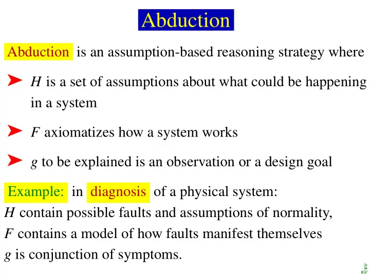
Abduction is an assumption-based reasoning strategy where

➤ H is a set of assumptions about what could be happening

in a system

➤ F axiomatizes how a system works ➤ g to be explained is an observation or a design goal

Example: in diagnosis of a physical system: H contain possible faults and assumptions of normality, F contains a model of how faults manifest themselves g is conjunction of symptoms.

☞ ☞

Abduction versus Default Reasoning

Abduction differs from default reasoning in that:

➤ The explanations are of interest, not just the conclusion. ➤ H contains assumptions of abnormality as well as

assumptions of normality.

➤ We don’t only explain normal outcomes. Often we want

to explain why some abnormal observation occurred.

➤ We don’t care if ¬g can also been explained.

☞ ☞ ☞

Abductive Diagnosis

➤ You need to axiomatize the effects of normal conditions

and faults.

➤ We need to be able to explain all of the observations. ➤ Assumables are all of those hypotheses that require no

further explanation.

☞ ☞ ☞

Electrical Environment

light two-way switch switch

• ff
• n

power

• utlet

circuit breaker

• utside power

l1 l2 w1 w0 w2 w4 w3 w6 w5 p2 p1 cb2 cb1 s1 s2 s3

☞ ☞ ☞

lit(L) ⇐ light(L) & ok(L) & live(L). dark(L) ⇐ light(L) & broken(L). dark(L) ⇐ light(L) & dead(L). live(W) ⇐ connected_to(W, W1) & live(W1). dead(W) ⇐ connected_to(W, W1) & dead(W1). dead(W) ⇐ unconnected(W). connected_to(l1, w0) ⇐ true. connected_to(w0, w1) ⇐ up(s2) & ok(s2). unconnected(w0) ⇐ broken(s2). unconnected(w1) ⇐ broken(s1). unconnected(w1) ⇐ down(s1). false ← ok(X) ∧ broken(X). assumable ok(X), broken(X), up(X), down(X).

☞ ☞ ☞

Explaining Observations

➤ To explain lit(l1) there are two explanations:

{ok(l1), ok(s2), up(s2), ok(s1), up(s1), ok(cb1)} {ok(l1), ok(s2), down(s2), ok(s1), down(s1), ok(cb1)}

➤ To explain lit(l2) there is one explanation:

{ok(cb1), ok(s3), up(s3), ok(l2)}

☞ ☞ ☞

Explaining Observations (cont)

➤ To explain dark(l1) there are 8 explanations:

{broken(l1)} {broken(cb1), ok(s1), up(s1), ok(s2), up(s2)} {broken(s1), ok(s2), up(s2)} {down(s1), ok(s2), up(s2)} {broken(cb1), ok(s1), down(s1), ok(s2), down(s2)} {up(s1), ok(s2), down(s2)} {broken(s1), ok(s2), down(s2)} {broken(s2)}

☞ ☞ ☞

Explaining Observations (cont)

➤ To explain dark(l1) ∧ lit(l2) there are explanations:

{ok(cb1), ok(s3), up(s3), ok(l2), broken(l1)} {ok(cb1), ok(s3), up(s3), ok(l2), broken(s1), ok(s2), up(s2)} {ok(cb1), ok(s3), up(s3), ok(l2), down(s1), ok(s2), up(s2)} {ok(cb1), ok(s3), up(s3), ok(l2), up(s1), ok(s2), down(s2)} {ok(cb1), ok(s3), up(s3), ok(l2), broken(s1), ok(s2), down(s2 {ok(cb1), ok(s3), up(s3), ok(l2), broken(s2)}

☞ ☞ ☞

Abduction for User Modeling

Suppose the infobot wants to determine what a user is interested in. We can hypothesize the interests of users: H = {interested_in(Ag, Topic)}. Suppose the corresponding facts are: selects(Ag, Art) ← about(Art, Topic) ∧ interested_in(Ag, Topic). about(art_94, ai). about(art_94, info_highway). about(art_34, ai). about(art_34, skiing).

☞ ☞ ☞

Explaining User’s Actions

There are two minimal explanations of selects(fred, art_94): {interested_in(fred, ai)}. {interested_in(fred, information_highway)}. If we observe selects(fred, art_94) ∧ selects(fred, art_34), there are two minimal explanations: {interested_in(fred, ai)}. {interested_in(fred, information_highway), interested_in(fred, skiing)}.

☞ ☞ ☞

Image interpretation

➤ A scene is the world that the agent is in. ➤ An image is what the agent sees. ➤ Vision: given an image try to determine the scene. ➤ Typically we know more about the scene → image

mapping than the image → scene mapping.

☞ ☞ ☞

Example Scene and Image Scene Image

☞ ☞ ☞

Scene and Image Primitives

Scene Primitives Image Primitives land, water region river, road, shore chain joins(X, Y, E)

X Y

tee (E ∈ {0, 1} specifies which end of X) mouth(X, Y, E)

X Y

cross(X, Y)

X Y

chi

☞ ☞ ☞

Scene and image primitives (cont.)

Scene Primitives Image Primitives beside(C, R)

C R

bounds(C,R) source(C, E)

C E

• pen(C,E)

loop(C)

C

closed(C) inside(C, R)

C R

interior(C,R)

• utside(C, R)

C R

exterior(C,R)

☞ ☞ ☞

Axiomatizing the Scene → Image map

chain(X) ← river(X) ∨ road(X) ∨ shore(X). region(X) ← land(X) ∨ water(X). tee(X, Y, E) ← joins(X, Y, E) ∨ mouth(X, Y, E). chi(X, Y) ← cross(X, Y).

• pen(X, N) ← source(X, N).

closed(X) ← loop(X). interior(X, Y) ← inside(X, Y). exterior(X, Y) ← outside(X, Y). assumable road(X), river(X), shore(X), land(X), . . . assumable joins(X, Y, E), cross(X, Y), mouth(L, R, E) . . .

☞ ☞ ☞

Scene Constraints

false ← cross(X, Y) ∧ river(X) ∧ river(Y). false ← cross(X, Y) ∧ (shore(X) ∨ shore(Y)). false ← mouth(R, L1, 1) ∧ river(R) ∧ mouth(R, L2, 0). start(R, N) ← river(R) ∧ road(Y) ∧ joins(R, Y, N). start(X, Y) ← source(X, Y). false ← start(R, 1) ∧ river(R) ∧ start(R, 0). false ← joins(R, L, N) ∧ river(R) ∧ (river(L) ∨ shore(L)). false ← mouth(X, Y, N) ∧ (road(X) ∨ road(Y)). false ← source(X, N) ∧ shore(X). false ← joins(X, A, N) ∧ shore(X). false ← loop(X) ∧ river(X).

☞ ☞ ☞

Scene constraints (continued)

false ← shore(X) ∧ inside(X, Y) ∧ outside(X, Z) ∧ land(Y) ∧ land(Z). false ← shore(X) ∧ inside(X, Y) ∧ outside(X, Z) ∧ water(Z) ∧ water(Y). false ← water(Y) ∧ beside(X, Y) ∧ (road(X) ∨ river(X)).

☞ ☞ ☞

Describing an image

1 c1 c2 r2 r1 chain(c1) ∧ chain(c2) ∧ region(r1) ∧ region(r2) ∧ tee(c2, c1, 1) ∧ bounds(c2, r2) ∧ bounds(c1, r1) ∧ bounds(c1, r2) ∧ interior(c1, r1) ∧ exterior(c1, r2) ∧ open(c2, 0) ∧ closed(c1)

☞ ☞ ☞

A more complicated image

1 1 1 c6 c5 c1 c2 c3 c4 r3 r4 r2 r1 1

chain(c1) ∧ open(c1, 0) ∧

• pen(c1, 1) ∧ region(r1) ∧

bounds(c1, r1) ∧ chain(c2) ∧ tee(c2, c1, 0) ∧ bounds(c2, r1) ∧ chain(c3) ∧ bounds(c3, r1) ∧ region(r2) ∧ bounds(c3, r2) ∧ chain(c5) ∧ closed(c5) ∧ bounds(c5, r2) ∧ exterior(c5, r2) ∧ region(r3) ∧ bounds(c5, r3) ∧ interior(c5, r3) ∧ …

☞ ☞ ☞

Parameterizing Assumables

Suppose we had a battery b connected to voltage meter: To be able to explain a measurement of the battery voltage, we need to parameterize the assumables enough: assumable flat(B, V). assumable tester_ok. measured_voltage(B, V) ← flat(B, V) ∧ tester_ok. false ← flat(B, V) ∧ V > 1.2.

☞ ☞