Ab initio methods: how/why do they work D.Svergun Small-angle - - PDF document

29-Oct-14 1

Ab initio methods: how/why do they work

D.Svergun

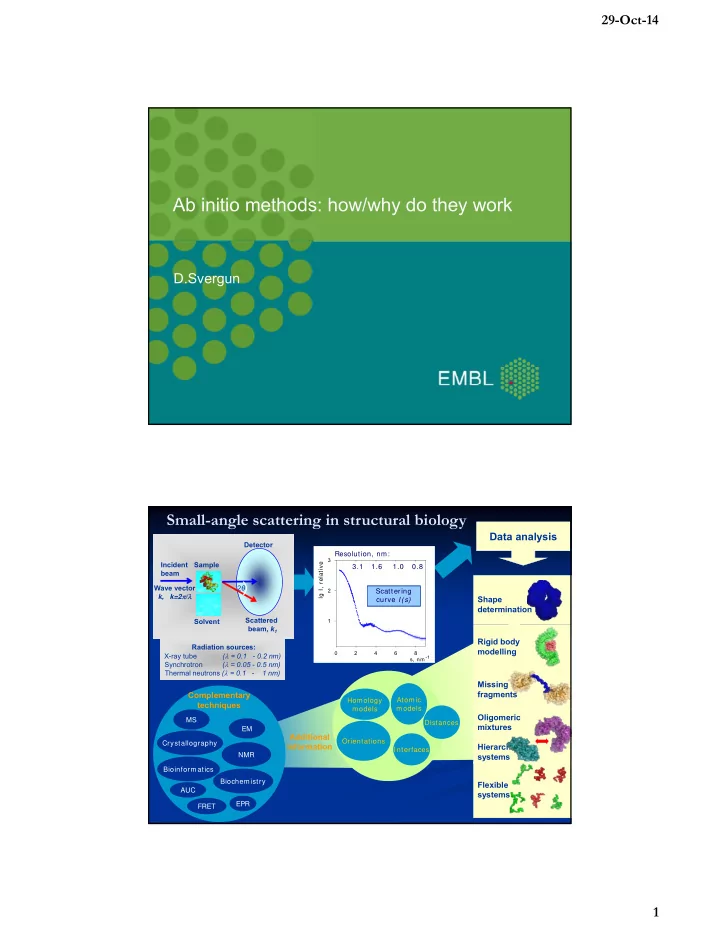
EM Crystallography NMR Biochemistry FRET Bioinformatics

Complementary techniques

AUC

Oligomeric mixtures Hierarchical systems Shape determination Flexible systems Missing fragments Rigid body modelling

Data analysis

Radiation sources: X-ray tube ( = 0.1 - 0.2 nm) Synchrotron ( = 0.05 - 0.5 nm) Thermal neutrons ( = 0.1 - 1 nm) Homology models Atomic models Orientations Interfaces

Additional information

2θ Sample Solvent Incident beam Wave vector k, k=2/ Detector Scattered beam, k1 EPR

Small-angle scattering in structural biology

s, nm -1 2 4 6 8

lg I, relative

1 2 3

Scattering curve I(s) Resolution, nm: 3.1 1.6 1.0 0.8 MS Distances

29-Oct-14 2

Major problem for biologists using SAS

• In the past, many biologists did

not believe that SAS yields more than the radius of gyration

• Now, an immensely grown

number of users are attracted by new possibilities of SAS and they want rapid answers to more and more complicated Questions

• The users often have to

perform numerous cumbersome actions during the experiment and data analysis, to become each of the Answers

Now we shall go through the major steps required on the way

Step 1: know, which units are used

The momentum transfer [q, Q, s, h, μ, κ …] = 4π sin(θ)/λ, I(s)=I0*exp(-sRg/3), sRg <1.3 [s, S, k, … ] = 2 sin(θ)/λ I(s)=I0*exp(-2πsRg/3), sRg <1.3*2π GNOM or CRYSOL input: Angular units in the input file: 4*pi*sin(theta)/lambda [1/angstrom] (1) 4*pi*sin(theta)/lambda [1/nm] (2) 2 * sin(theta)/lambda [1/angstrom] (3) 2 * sin(theta)/lambda [1/nm] (4)

s, nm -1 2 4 6 8

lg I, relative

1 2 3

Scattering curve I(s) Resolution, nm: 3.1 1.6 1.0 0.8

29-Oct-14 3

Scattering from dilute macromolecular solutions (monodisperse systems)

dr sr sr r p s I

D



 sin ) ( 4 ) ( 

The scattering is proportional to that

• f a single particle averaged over all
• rientations,

which allows

• ne

to determine size, shape and internal structure of the particle at low (1-10 nm) resolution.

Sample and buffer scattering

29-Oct-14 4

Overall parameters

) s R ) I( I(s)

g 2 2

3 1 exp(  

Radius of gyration Rg (Guinier, 1939) Maximum size Dmax: p(r)=0 for r> Dmax Excluded particle volume (Porod, 1952)





 

2 2

) ( I(0)/Q; 2 V ds s I s Q 

Molecular mass (from I(0))

The scattering is related to the shape (or low resolution structure)

s, nm-1

0.0 0.1 0.2 0.3 0.4 0.5

lg I(s), relative

• 6
• 5
• 4
• 3
• 2
• 1

Solid sphere Long rod Flat disc Hollow sphere Dumbbell

s, nm-1

0.0 0.1 0.2 0.3 0.4 0.5

lg I(s), relative

• 6
• 5
• 4
• 3
• 2
• 1

s, nm-1

0.0 0.1 0.2 0.3 0.4 0.5

lg I(s), relative

• 6
• 5
• 4
• 3
• 2
• 1

s, nm-1

0.0 0.1 0.2 0.3 0.4 0.5

lg I(s), relative

• 6
• 5
• 4
• 3
• 2
• 1

s, nm-1

0.0 0.1 0.2 0.3 0.4 0.5

lg I(s), relative

• 6
• 5
• 4
• 3
• 2
• 1

29-Oct-14 5

Shape determination: how?

Lack of 3D information inevitably leads to ambiguous interpretation, and additional information is always required

3D search model

M parameters

Non-linear search

1D scattering data

Trial-and-error

Ab initio methods

Advanced methods of SAS data analysis employ spherical harmonics (Stuhrmann, 1970) instead of Fourier transformations

29-Oct-14 6

The use of spherical harmonics

SAS intensity is I(s) = <I(s)> = <{F [(r)]}2>, where F denotes the Fourier transform, <> stands for the spherical average, and s=(s, ) is the scattering vector. Expanding (r) in spherical harmonics

) ( ) ( ) (   

lm lm l l m l

Y r

 

   

 r

the scattering intensity is expressed as

I s A s

l m l l lm

( ) ( ) 

  

 

2

2 2



where the partial amplitudes Alm(s) are the Hankel transforms from the radial functions

A s i r j sr r dr

lm l lm l

( ) ( ) ( ) 





2

2

 

and jl(sr) are the spherical Bessel functions.

Stuhrmann, H.B. Acta Cryst., A26 (1970) 297.

Structure of bacterial virus T7

Svergun, D.I., Feigin, L.A. & Schedrin, B.M. (1982) Acta Cryst. A38, 827 Agirrezabala, J. M. et al. & Carrascosa J.L. (2005) EMBO J. 24, 3820 SAXS, 1982 Cryo-EM, 2005 Pro-head Mature virus

29-Oct-14 7

Ylm() – orthogonal spherical harmonics, flm – parametrization coefficients,

Small-angle scattering intensity from the entire particle is calculated as the sum of scattering from partial harmonics:

 

  

  

L L

Y f F F ) ( ) ( ) (

l l l m lm lm

  

Shape parameterization by spherical harmonics

Homogeneous particle Scattering density in spherical coordinates (r,) = (r,,) may be described by the envelope function:

) ( ) ( , , 1 ) (    F r F r        r

Shape parameterization by a limited series of spherical harmonics:

 

  



L theor

s A s I

2 2

) ( 2 ) (

l l l m lm



Stuhrmann, H. B. (1970) Z.

• Physik. Chem. Neue Folge 72,

177-198. Svergun, D.I. et al. (1996) Acta

• Crystallogr. A52, 419-426.

F() is an envelope function

r 

Homogeneous particle

f00 A00(s) = + f11 + + A11(s) +

• f20

+ A20(s) +

• +

f22 + A22(s) +

• +

+…

Spatial resolution: , R – radius of an equivalent sphere. Number of model parameters flm is (L+1)2. One can easily impose symmetry by selecting appropriate harmonics in the sum. This significantly reduces the number of parameters describing F() for a given L.

) 1 ( π   L R 

F() is an

envelope function

r 

Shape parameterization by spherical harmonics

29-Oct-14 8

Program SASHA

Vector of model parameters: Position ( j ) = x( j ) = (phase assignments)

Number of model parameters M  (Dmax / r0)3  103 is too big for conventional minimization methods – Monte-Carlo like approaches are to be used

But: This model is able to describe rather complex shapes

Chacón, P. et al. (1998) Biophys. J. 74, 2760-2775. Svergun, D.I. (1999) Biophys. J. 76, 2879-2886

Solvent Particle

2r0

A sphere of radius Dmax is filled by densely packed beads of radius r0<< Dmax

Dmax

   solvent if particle if 1

Bead (dummy atoms) model

29-Oct-14 9

Finding a global minimum

Pure Monte Carlo runs in a danger to be trapped into a local minimum Solution: use a global minimization method like simulated annealing or genetic algorithm

Local and global search on the Great Wall

Local search always goes to a better point and can thus be trapped in a local minimum Pure Monte-Carlo search always goes to the closest local minimum (nature: rapid quenching and vitreous ice formation) To get out of local minima, global search must be able to (sometimes) go to a worse point Slower annealing allows to search for a global minimum (nature: normal, e.g. slow freezing of water and ice formation)

29-Oct-14 10

Aim: find a vector of M variables {x} minimizing a function f(x) 1. Start from a random configuration x at a “high” temperature T. 2. Make a small step (random modification of the configuration) x  x’ and compute the difference  = f(x’) - f(x). 3. If  < 0, accept the step; if  > 0, accept it with a probability e-  /T 4. Make another step from the old (if the previous step has been rejected)

• r from the new (if the step has been accepted) configuration.

5. Anneal the system at this temperature, i.e. repeat steps 2-4 “many” (say, 100M tries or 10M successful tries, whichever comes first) times, then decrease the temperature (T’ = cT, c<1). 6. Continue cooling the system until no improvement in f(x) is observed. Shape determination: M≈ 103 variables (e.g. 0 or 1 bead assignments in DAMMIN Rigid body methods: M≈ 101 variables (positional and rotational parameters

• f the subunits)

f(x) is always (Discrepancy + Penalty)

Simulated annealing Ab initio program DAMMIN

Using simulated annealing, finds a compact dummy atoms configuration X that fits the scattering data by minimizing where  is the discrepancy between the experimental and calculated curves, P(X) is the penalty to ensure compactness and connectivity, > 0 its weight.

) ( )] , ( ), ( [ ) (

exp 2

X P X s I s I X f    

compact loose disconnected

29-Oct-14 11

Why/how do ab initio methods work

The 3D model is required not only to fit the data but also to fulfill (often stringent) physical and/or biochemical constrains

Why/how do ab initio methods work

The 3D model is required not only to fit the data but also to fulfill (often stringent) physical and/or biochemical constrains

29-Oct-14 12

A test ab initio shape determination run

Bovine serum albumin, molecular mass 66 kDa, no symmetry imposed Program DAMMIN Slow mode

A test ab initio shape determination run

Program DAMMIN Slow mode Bovine serum albumin: comparison of the ab initio model with the crystal structure of human serum albumin

29-Oct-14 13

DAMMIF, a fast DAMMIN

DAMMIF is a completely reimplemented DAMMIN written in object-oriented code

• About 25-40 times faster

than DAMMIN (in fast mode, takes about 1-2 min

• n a PC)
• Employs adaptive search

volume

• Makes use of multiple

CPUs

Franke, D. & Svergun, D. I. (2009)

• J. Appl. Cryst. 42, 342–346

Limitations of shape determination

 Very low resolution  Ambiguity of the models

s, nm-1 5 10 15 lg I(s) 5 6 7 8 Resolution, nm 2.00 1.00 0.67 0.50 0.33

Shape F

• ld

Atomic structure

How to construct ab initio models accounting for higher resolution data? Accounts for a restricted portion of the data

29-Oct-14 14

Ab initio dummy residues model

 Proteins

typically consist

• f

folded polypeptide chains composed of amino acid residues Scattering from such a model is computed using the Debye (1915) formula. Starting from a random model, simulated annealing is employed similar to DAMMIN At a resolution

• f

0.5 nm a protein can be represented by an ensemble of K dummy residues centered at the C positions with coordinates { ri}

Distribution of neighbors

Excluded volume effects and local interactions lead to a characteristic distribution of nearest neighbors around a given residue in a polypeptide chain

Shell radius, nm 0.2 0.4 0.6 0.8 1.0 Number of neighbours 1 2 3 4 5 6

29-Oct-14 15

GASBOR run on C subunit of V-ATPase

Starting from a random “gas”

• f 401 dummy

residues, fits the data by a locally chain- compatible model

Beads: Ambruster et al. (2004, June) FEBS Lett. 570, 119 Cα trace: Drory et al. (2004, November), EMBO reports, 5, 1148

GASBOR run on C subunit of V-ATPase

29-Oct-14 16

Benchmarking ab initio methods

s, nm-1 5 10 log I, relative 1 2 Experimental data Envelope model Bead model Dummy residue model

Comparison with the crystal SASHA DAMMI N GASBOR structure of lysozyme 1996 1999 2001 Envelope Bead model Dummy residues

Z M

1.2 m

N C

Z-disc I-band A-band H-zone

26 926 aa

I27 FNIII TK M5

Z

Z1Z2 Z7 I1 I27 Ax TK M5 fold IG EF IG IG FN-III kinase IG method X NMR X NMR NMR X NMR

NMR data: Pastore lab; X-ray data: Wilmanns lab

Modular structure of a giant mucsle protein titin

29-Oct-14 17

Native Z1Z2 His-Z1Z2 Tele90-Z1Z2



Z1Z2 includes two modules at the N-terminal of the Z-disc of titin and interacts with telethonin

Solution structure of Z1Z2-telethonin complex

Zou, P ., Gautel, M., Geerlof, M., Wilmanns, M., Koch, M.H.J. & Svergun, D.I. (2003)

• J. Biol. Chem. 278, 2636

Shape of Z1Z2 and localization of the his-tag Cross-linking function

• f telethonin

Crystal structure of Z1Z2-telethonin complex

~100 Å

Zou P ., Pinotsis N., Lange S., Song Y .H., Popov A., Mavridis I., Mayans O.M., Gautel M. & Wilmanns M. (2006) Nature 439, 229-33.

29-Oct-14 18

Shape analysis for multi-component systems: principle

One component, one scattering pattern: “normal” shape determination

Chacón, P . et al. (1998) Biophys. J. 74, 2760-2775 Svergun, D.I. (1999) Biophys. J. 76, 2879-2886

Shape analysis for multi-component systems: principle

Many components, many scattering patterns: shape and internal structure

Svergun, D.I. (1999) Biophys. J. 76, 2879-2886 Svergun, D.I. & Nierhaus, K.H. (2000) J. Biol. Chem. 275, 14432-14439

A+ B A B

29-Oct-14 19

EGC stator sub-complex of V-ATPase

Diepholz, M. et al. (2008) Structure 16, 1789-1798

In solution, EG makes an L-shaped assembly with subunit-C. This model is supported by the EM showing three copies of EG, two of them linked by C. The data further indicate a conformational change of EGC during regulatory assembly/disassembly.

EG+ C C subunit EG subunit Scattering from free subunits and their complex in solution

3D map of the yeast V-ATPase by electron microscopy.

Ab initio shapes

Scattering from a multiphase particle

s, nm-1

0.5 1.0 1.5 2.0

lg I, relative

8 9 10 11 0% D2O 40% D2O 55% D2O 75% D2O 100% D2O

 



    

k j jk m i m j j j m j m

s I s I s I ) ( 2 ) ( ) ( ) (

2

  

29-Oct-14 20

Ab initio multiphase modelling

Start: random phase assignments within the search volume, no fit to the experimental data Finish: condensed multiphase model with minimum interfacial area fitting multiple data sets

Program MONSA, Svergun, D.I. (1999) Biophys. J. 76, 2879; Petoukhov, M.V. & Svergun, D. I. (2006) Eur. Biophys. J. 35, 567.

Ternary complex: Exportin-t/Ran/tRNA

Ran (structure known) Exportin-t t-RNA (structure known) (tentative homology model)

29-Oct-14 21

X-rays: ab initio overall shape

s, nm-1

0.5 1.0 1.5 2.0

lg I, relative

5 6 7 8 Ternary complex Ran tRNA Fits

One X-ray scattering pattern from the ternary complex fitted by DAMMIN

Fukuhara, N., Fernandez, E., Ebert, J., Conti, E. & Svergun, D. I. (2004) J. Biol. Chem. 279, 2176

Scattering data from Exportin-t/Ran/tRNA

X-ray scattering



From Exportin-t, Ran, tRNA 3 curves

Neutron scattering



Ternary complex with protonated Ran in 0, 40, 55, 75, 100% D2O 5 curves



Ternary complex with deuterated Ran in 0, 40, 55, 70, 100% D2O 5 curves

TOTAL 13 curves

29-Oct-14 22

Contrast variation: localization of tRNA

s, nm-1

0.5 1.0 1.5 2.0

lg I, relative

5 6 7 8 Ternary complex Ran tRNA Fits

s, nm-1

0.5 1.0 1.5 2.0

lg I, relative

8 9 10 11 0% D2O 40% D2O 55% D2O 75% D2O 100% D2O Fits

Three X-ray and five neutron data sets fitted by MONSA

Specific deuteration: highlighting d-Ran

s, nm-1

0.5 1.0 1.5 2.0

lg I, relative

5 6 7 8 Ternary complex Ran tRNA Fits

s, nm-1

0.5 1.0 1.5 2.0

lg I, relative

8 9 10 11 0% D2O 40% D2O 55% D2O 75% D2O 100% D2O Fits

s, nm-1

0.5 1.0 1.5 2.0

lg I, relative

9 10 11 0% D2O 40% D2O 55% D2O 70% D2O 100% D2O Fits

Three X-ray and ten neutron data sets fitted by MONSA

29-Oct-14 23

Ternary complex: Exportin-t/Ran/tRNA

s, nm-1

0.5 1.0 1.5 2.0

lg I, relative

5 6 7 8 Ternary complex Ran tRNA Fits

s, nm-1

0.5 1.0 1.5 2.0

lg I, relative

8 9 10 11 0% D2O 40% D2O 55% D2O 75% D2O 100% D2O Fits

s, nm-1

0.5 1.0 1.5 2.0

lg I, relative

9 10 11 0% D2O 40% D2O 55% D2O 70% D2O 100% D2O Fits

High resolution models of the components docked into the three-phase ab initio model of the complex based on X-ray and neutron scattering from selectively deuterated particles

Shapes from recent projects at EMBL-HH

Domain and quaternary structure Complexes and assemblies Structural transitions Flexible/transient systems

Bernado et al JMB (2008) Src kinase She et al, Mol Cell (2008) Dcp1/Dcp2 complex Xu et al JACS (2008) Cytochrome/adrenodoxin Fagan et al Mol. Microbiol (2009) S-layer proteins Albesa-Jové et al JMB (2010) Toxin B Giehm et al PNAS USA (2011) α-synuclein oligomers Complement factor H Morgan et al NSMB (2011)

29-Oct-14 24

Ab initio programs for SAS

 Genetic algorithm DALAI_GA (Chacon et al., 1998, 2000)  ‘Give-n-take’ procedure SAXS3D (Bada et al., 2000)  Spheres modeling program GA_STRUCT (Heller et al., 2002)  Envelope models: SASHA(1) (Svergun et al., 1996)  Dummy atoms: DAMMIN(1,4) & MONSA(1,2) (Svergun, 1999)  Dummy residues: GASBOR(1,3) (Petoukhov et al., 2001)

(1) Able to impose symmetry and anisometry constrains (2) Multiphase inhomogeneous models (3) Accounts for higher resolution data (4) DAMMIF is 30 times faster (D.Franke & D.Svergun, 2009)

Some words of caution

Or Always remember about ambiguity!

29-Oct-14 25

Shape determination of 5S RNA: a variety of DAMMIN models yielding identical fits

Funari, S., Rapp, G., Perbandt, M., Dierks, K., Vallazza, M., Betzel, Ch., Erdmann, V. A. & Svergun, D. I. (2000) J. Biol. Chem. 275, 31283-31288.

Kozin, M.B. & Svergun, D.I. (2001) J. Appl. Crystallogr. 34, 33-41

Program SUPCOMB – a tool to align and conquer

 Aligns heterogeneous high- and low-resolution models and

provides a dissimilarity measure (NSD)

 For shape determination, allows one to find common

features in a series of independent reconstructions

29-Oct-14 26

1. Find a set of solutions starting from random initial models and superimpose all pairs of models with SUPCOMB. 2. Find the most probable model (which is on average least different from all the others) and align all the other models with this reference

• ne.

3. Remap all models onto a common grid to obtain the solution spread region and compute the spatial occupancy density of the grid points. 4. Reduce the spread region by rejecting knots with lowest occupancy to find the most populated volume 5. These steps are automatically done by a package called DAMAVER if you just put all multiple solutions in one directory

Automated analysis of multiple models

Program DAMAVER, Volkov & Svergun (2003) J. Appl. Crystallogr. 36, 860

5S RNA: ten shapes superimposed

Solution spread region Solution spread region

29-Oct-14 27

5S RNA: ten shapes superimposed

Most populated volume Most populated volume

5S RNA: final solution

The final model obtained within the solution spread region The final model obtained within the solution spread region

29-Oct-14 28

0.0 0.2 0.4 0.6 0.8 1.0 10

• 4

10

• 3

10

• 2

10

• 1

10

s I

data SASHA DAMMIN

Stable solutions

0.0 0.2 0.4 0.6 0.8 1.0 10

• 3

10

• 2

10

• 1

10

s I

data SASHA DAMMIN 0.0 0.1 0.2 0.3 0.4 10

10

10

10

s I

data SASHA DAMMIN

cylinder 2:5 cylinder 2:5 cube cube Prism 1:2:4 Prism 1:2:4

Spread region Most probable volume Spread region Most probable volume Average NSD ≈ 0.5 Average NSD ≈ 0.5

Uniqueness of ab initio analysis Fair stability

0.0 0.1 0.2 0.3 10

10

s I

data SASHA DAMMIN 0.0 0.1 0.2 0.3 10

10

10

10

s I

data body 1 body 2

3

1

1

cylinder 1:10 cylinder 1:10 Ring 1:3:1 Ring 1:3:1

Spread region Most probable volume Spread region Most probable volume Spread region Most probable volume Spread region Most probable volume Average NSD ≈ 0.9 Average NSD ≈ 0.9 Volkov, V .V . & Svergun, D.I. (2003) J. Appl. Crystallogr. 36, 860-864.

29-Oct-14 29

0.0 0.1 0.2 0.3 10

10

10

10

10

s I

data SASHA DAMMIN 0.0 0.1 0.2 0.3 10

10

s I

data SASHA DAMMIN

Poor stability

Spread region Most probable volume Spread region Most probable volume Spread region Most probable volume Spread region Most probable volume

Disk 10:1 Disk 10:1 Disk 5:1 Disk 5:1

Very long search may provide more accurate model Very long search may provide more accurate model This structure can not be restored without use of additional information This structure can not be restored without use of additional information Average NSD > 1 Average NSD > 1

Use of symmetry

Original body Original body Typical solution with P5 symmentry Typical solution with P5 symmentry Typical solution with no symmetry Typical solution with no symmetry Spread region Most probable volume Spread region Most probable volume

However: symmetry biases the results and must also be used with caution. Always run in P1 first! However: symmetry biases the results and must also be used with caution. Always run in P1 first!

29-Oct-14 30

Shape determination of V1 ATPase

P1 P3 P3, prolate

Svergun, D.I., Konrad, S., Huss, M., Koch, M.H.J., Wieczorek, H., Altendorf, K.- H., Volkov, V .V . & Grueber, G. (1998) Biochemistry 37, 17659-17663.

Quantifying Inherent Ambiguity of SAS data

Exhaustive calculations of scattering by all (14112) possible skeletons represented by up to seven densely packed interconnected beads on a grid provided a map of ambiguity, i.e. the propensity that a given scattering pattern yields an ambiguous shape reconstruction

Map of SAXS profiles density

s*Rg

1 2 3 4 5 6

lg(I/I0)

• 1.6
• 1.2
• 0.8
• 0.4

0.0 10 100 1000 10000

Extreme cases

Flat Disc Rod Sphere

Petoukhov & Svergun, submitted

AMBIMETER

29-Oct-14 31

Progress in ab initio methods

2014 1993

And now let us awake for the practical work

 M.Petoukhov,

D.Franke:

Ab initio tutorial