Ab initio methods: how/why do they work D.Svergun, EMBL-Hamburg - - PDF document

Ab initio methods: how/why do they work

D.Svergun, EMBL-Hamburg

EM Crystallography NMR Biochemistry FRET Bioinformatics

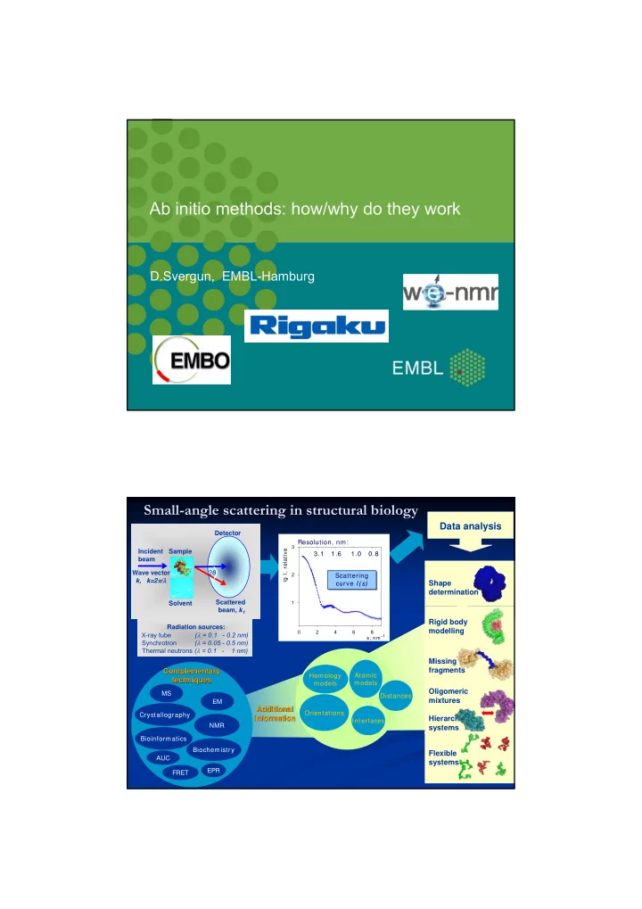
Complementary Complementary techniques techniques

AUC

Oligomeric mixtures Hierarchical systems Shape determination Flexible systems Missing fragments Rigid body modelling

Data analysis

Radiation sources: X-ray tube (λ = 0.1 - 0.2 nm) Synchrotron (λ = 0.05 - 0.5 nm) Thermal neutrons (λ = 0.1 - 1 nm) Homology models Atomic models Orientations Interfaces

Additional Additional information information

2θ Sample Solvent Incident beam Wave vector k, k=2π/λ Detector Scattered beam, k1 EPR

Small Small-

• angle scattering in structural biology

angle scattering in structural biology

s, nm -1 2 4 6 8

lg I, relative

1 2 3

Scattering curve I(s) Scattering curve I(s) Resolution, nm: 3.1 1.6 1.0 0.8 MS Distances

Major problem for biologists using SAS Major problem for biologists using SAS

• In the past, many biologists did

not believe that SAS yields more than the radius of gyration

• Now, an immensely grown

number of users are attracted by new possibilities of SAS and they want rapid answers to more and more complicated Questions

• The users often have to

perform numerous cumbersome actions during the experiment and data analysis, to become each of the Answers

Now we shall go through the major steps required on the way

Step 1: know, which units are used Step 1: know, which units are used

The momentum transfer [q, Q, s, h, μ, κ …] = 4π sin(θ)/λ, I(s)=I0*exp(-sRg/3), sRg <1.3 [s, S, k, … ] = 2 sin(θ)/λ I(s)=I0*exp(-2πsRg/3), sRg <1.3*2π GNOM or CRYSOL input: Angular units in the input file: 4*pi*sin(theta)/lambda [1/angstrom] (1) 4*pi*sin(theta)/lambda [1/nm] (2) 2 * sin(theta)/lambda [1/angstrom] (3) 2 * sin(theta)/lambda [1/nm] (4)

s, nm -1 2 4 6 8

lg I, relative

1 2 3

Scattering curve I(s) Scattering curve I(s) Resolution, nm: 3.1 1.6 1.0 0.8

Scattering from dilute macromolecular Scattering from dilute macromolecular solutions ( solutions (monodisperse monodisperse systems) systems)

dr sr sr r p s I

D

∫

= sin ) ( 4 ) ( π

The scattering is proportional to that

• f a single particle averaged over all
• rientations, which allows one to

determine size, shape and internal structure of the particle at low (1-10 nm) resolution.

Sample and buffer scattering Sample and buffer scattering

Overall parameters Overall parameters

) s R ) I( I(s)

g 2 2

3 1 exp( − ≅

Radius of gyration Rg (Guinier, 1939) Maximum size Dmax: p(r)=0 for r> Dmax Excluded particle volume (Porod, 1952)

∫

∞

= =

2 2

) ( I(0)/Q; 2 V ds s I s Q π

Molecular mass (from I(0))

The scattering is related to the shape The scattering is related to the shape (or low resolution structure) (or low resolution structure)

s, nm-1

0.0 0.1 0.2 0.3 0.4 0.5

lg I(s), relative

• 6
• 5
• 4
• 3
• 2
• 1

Solid sphere Long rod Flat disc Hollow sphere Dumbbell

s, nm-1

0.0 0.1 0.2 0.3 0.4 0.5

lg I(s), relative

• 6
• 5
• 4
• 3
• 2
• 1

s, nm-1

0.0 0.1 0.2 0.3 0.4 0.5

lg I(s), relative

• 6
• 5
• 4
• 3
• 2
• 1

s, nm-1

0.0 0.1 0.2 0.3 0.4 0.5

lg I(s), relative

• 6
• 5
• 4
• 3
• 2
• 1

s, nm-1

0.0 0.1 0.2 0.3 0.4 0.5

lg I(s), relative

• 6
• 5
• 4
• 3
• 2
• 1

Shape determination: how? Shape determination: how?

Lack of 3D information Lack of 3D information inevitably leads to inevitably leads to ambiguous interpretation, ambiguous interpretation, and additional information is and additional information is always required always required

3D search model

M parameters

Non-linear search

1D scattering data

Trial-and-error

Ab initio Ab initio methods methods

Advanced methods of SAS data analysis employ spherical harmonics (Stuhrmann, 1970) instead of Fourier transformations

The use of spherical harmonics

SAS intensity is I(s) = <I(s)>Ω = <{F [ρ(r)]}2>Ω, where F denotes the Fourier transform, <>Ω stands for the spherical average, and s=(s, Ω) is the scattering vector. Expanding ρ(r) in spherical harmonics

) ( ) ( ) ( ω ρ ρ

lm lm l l m l

Y r

∑ ∑

− = ∞ =

= r

the scattering intensity is expressed as

I s A s

l m l l lm

( ) ( ) =

= ∞ =−

∑ ∑

2

2 2

π

where the partial amplitudes Alm(s) are the Hankel transforms from the radial functions

A s i r j sr r dr

lm l lm l

( ) ( ) ( ) =

∞

∫

2

2

π ρ

and jl(sr) are the spherical Bessel functions.

Stuhrmann, H.B. Acta Cryst., A26 (1970) 297.

Structure of bacterial virus T7 Structure of bacterial virus T7

Svergun, D.I., Feigin, L.A. & Schedrin, B.M. Svergun, D.I., Feigin, L.A. & Schedrin, B.M. (1982) (1982) Acta Cryst. Acta Cryst. A38 A38, 827 , 827 Agirrezabala, J. M. Agirrezabala, J. M. et al. et al. & Carrascosa J.L. (2005) & Carrascosa J.L. (2005) EMBO J. EMBO J. 24 24, 3820 , 3820 SAXS, 1982 SAXS, 1982 Cryo Cryo-

• EM, 2005

EM, 2005 Pro Pro-

• head

head Mature virus Mature virus

Ylm(ω) – orthogonal spherical harmonics, flm – parametrization coefficients,

Small-angle scattering intensity from the entire particle is calculated as the sum of scattering from partial harmonics:

∑ ∑

= − =

⋅ = ≅

L L

Y f F F ) ( ) ( ) (

l l l m lm lm

ω ω ω

Shape parameterization by spherical harmonics

Homogeneous particle Scattering density in spherical coordinates (r,ω) = (r,θ,ϕ) may be described by the envelope function:

) ( ) ( , , 1 ) ( ω ω ρ F r F r > ≤ ≤ ⎩ ⎨ ⎧ = r

Shape parameterization by a limited series of spherical harmonics:

∑ ∑

= − =

=

L theor

s A s I

2 2

) ( 2 ) (

l l l m lm

π

Stuhrmann, H. B. (1970) Z.

• Physik. Chem. Neue Folge 72,

177-198. Svergun, D.I. et al. (1996) Acta

• Crystallogr. A52, 419-426.

F(ω) is an envelope function

r ρ

Homogeneous particle

f00 A00(s) = + f11 + + A11(s) +

• f20

+ A20(s) +

• +

f22 + A22(s) +

• +

+…

Spatial resolution: , R – radius of an equivalent sphere. Number of model parameters flm is (L+1)2. One can easily impose symmetry by selecting appropriate harmonics in the sum. This significantly reduces the number of parameters describing F(ω) for a given L.

) 1 ( π + = L R δ

F(ω) is an

envelope function

r ρ

Shape parameterization by spherical harmonics

Program SASHA Program SASHA

Vector of model parameters: Position ( j ) = x( j ) = (phase assignments)

Number of model parameters M ≈ (Dmax / r0)3 ≈ 103 is too big for conventional minimization methods – Monte-Carlo like approaches are to be used

But: This model is able to describe rather complex shapes

Chacón, P. et al. (1998) Biophys. J. 74, 2760-2775. Svergun, D.I. (1999) Biophys. J. 76, 2879-2886

Solvent Particle

2r0

A sphere of radius Dmax is filled by densely packed beads of radius r0<< Dmax

Dmax

⎩ ⎨ ⎧ solvent if particle if 1

Bead (dummy atoms) model Bead (dummy atoms) model

Finding a global minimum Finding a global minimum

Pure Monte Carlo runs in a danger to be trapped into a Pure Monte Carlo runs in a danger to be trapped into a local minimum local minimum Solution: use a global minimization method like Solution: use a global minimization method like simulated annealing or genetic algorithm simulated annealing or genetic algorithm

Local and global search on the Great Wall Local and global search on the Great Wall

L

• c

a l Local search always goes to a better Local search always goes to a better point and can thus be trapped in a local point and can thus be trapped in a local minimum minimum Pure Monte Pure Monte-

• Carlo search always goes to

Carlo search always goes to the closest local minimum (nature: rapid the closest local minimum (nature: rapid quenching and vitreous ice formation) quenching and vitreous ice formation) Global Global To get out of local minima, global search To get out of local minima, global search must be able to (sometimes) go to a must be able to (sometimes) go to a worse point worse point Slower annealing allows to search for a Slower annealing allows to search for a global minimum (nature: normal, e.g. global minimum (nature: normal, e.g. slow freezing of water and ice formation) slow freezing of water and ice formation)

Aim: find a vector of M variables {x} minimizing a function f(x) 1. Start from a random configuration x at a “high” temperature T. 2. Make a small step (random modification of the configuration) x → x’ and compute the difference Δ = f(x’) - f(x). 3. If Δ < 0, accept the step; if Δ > 0, accept it with a probability e- Δ /T 4. Make another step from the old (if the previous step has been rejected)

• r from the new (if the step has been accepted) configuration.

5. Anneal the system at this temperature, i.e. repeat steps 2-4 “many” (say, 100M tries or 10M successful tries, whichever comes first) times, then decrease the temperature (T’ = cT, c<1). 6. Continue cooling the system until no improvement in f(x) is observed. Shape determination: M≈ 103 variables (e.g. 0 or 1 bead assignments in DAMMIN Rigid body methods: M≈ 101 variables (positional and rotational parameters

• f the subunits)

f(x) is always (Discrepancy + Penalty)

Simulated annealing Simulated annealing Ab Ab initio initio program DAMMIN program DAMMIN

Using simulated annealing, finds a compact dummy Using simulated annealing, finds a compact dummy atoms configuration X that fits the scattering data by atoms configuration X that fits the scattering data by minimizing minimizing where where χ

χ is the discrepancy between the experimental

is the discrepancy between the experimental and calculated curves, and calculated curves, P(X) P(X) is the penalty to ensure is the penalty to ensure compactness and connectivity, compactness and connectivity, α

α> 0

> 0 its weight. its weight.

) ( )] , ( ), ( [ ) (

exp 2

X P X s I s I X f α χ + =

compact compact loose loose disconnected disconnected

Why/how do Why/how do ab initio ab initio methods work methods work

The 3D model is required not only to fit the data but also to fulfill (often stringent) physical and/or biochemical constrains

Why/how do Why/how do ab initio ab initio methods work methods work

The 3D model is required not only to fit the data but also to fulfill (often stringent) physical and/or biochemical constrains

A test A test ab initio ab initio shape determination run shape determination run

Bovine serum albumin, molecular mass 66 kDa, no symmetry imposed Program DAMMIN Slow mode

A test A test ab initio ab initio shape determination run shape determination run

Program DAMMIN Slow mode Bovine serum albumin: comparison of the ab initio model with the crystal structure of human serum albumin

DAMMIF, a fast DAMMIN DAMMIF, a fast DAMMIN

DAMMIF is a completely reimplemented DAMMIN written in object-oriented code

• About 25-40 times faster

than DAMMIN (in fast mode, takes about 1-2 min

• n a PC)
• Employs adaptive search

volume

• Makes use of multiple

CPUs

Franke, D. & Svergun, D. I. (2009)

• J. Appl. Cryst. 42, 342–346

Limitations of shape determination Limitations of shape determination

• Very low resolution

Very low resolution

• Ambiguity of the models

Ambiguity of the models

s, nm-1 5 10 15 lg I(s) 5 6 7 8 Resolution, nm 2.00 1.00 0.67 0.50 0.33

Shape F

• ld

Atomic structure

How to construct ab initio models accounting for higher resolution data? Accounts for a restricted portion of the data

Ab initio Ab initio dummy residues model dummy residues model

• Proteins

Proteins typically consist of folded polypeptide typically consist of folded polypeptide chains composed of amino acid residues chains composed of amino acid residues Scattering from such a model is computed using the Debye (1915) formula. Starting from a random model, simulated annealing is employed similar to DAMMIN At a resolution of 0.5 nm a protein can be represented by an ensemble of K dummy residues centered at the Cα positions with coordinates { ri}

Distribution of neighbors

Excluded volume effects and local interactions lead to a characteristic distribution of nearest neighbors around a given residue in a polypeptide chain

Shell radius, nm 0.2 0.4 0.6 0.8 1.0 Number of neighbours 1 2 3 4 5 6

GASBOR run on C subunit of V GASBOR run on C subunit of V-

• ATPase

ATPase

Starting from a random “gas”

• f 401 dummy

residues, fits the data by a locally chain- compatible model

Beads: Ambruster Beads: Ambruster et al. et al. (2004, June) (2004, June) FEBS Lett. 570, 119 Cα trace: Drory et al. (2004, November), EMBO reports, 5, 1148

GASBOR run on C subunit of V GASBOR run on C subunit of V-

• ATPase

ATPase

Benchmarking Benchmarking ab initio ab initio methods methods

s, nm-1 5 10 log I, relative 1 2 Experimental data Envelope model Bead model Dummy residue model

Comparison with the crystal Comparison with the crystal SASHA SASHA DAMMI N DAMMI N GASBOR GASBOR structure structure of lysozyme

• f lysozyme 1996

1996 1999 1999 2001 2001 Envelope Envelope Bead model Bead model Dummy residues Dummy residues

Z M

1.2 μm

N C

Z-disc I-band A-band H-zone

26 926 aa

I27 FNIII TK M5

Z

Z1Z2 Z7 I1 I27 Ax TK M5 fold IG EF IG IG FN-III kinase IG method X NMR X NMR NMR X NMR

NMR data: Pastore lab; X-ray data: Wilmanns lab

Modular structure of a giant mucsle protein titin

Native Z1Z2 His-Z1Z2 Tele90-Z1Z2

• Z1Z2 includes two modules at the N

Z1Z2 includes two modules at the N-

• terminal of the Z

terminal of the Z-

• disc of titin and

disc of titin and interacts with telethonin interacts with telethonin

Solution structure of Z1Z2 Solution structure of Z1Z2-

• telethonin complex

telethonin complex

Zou, P., Gautel, M., Geerlof, M., Wilmanns, M., Koch, M.H.J. & Svergun, D.I. (2003)

• J. Biol. Chem. 278, 2636

Shape of Z1Z2 and localization of the his-tag Cross-linking function

• f telethonin

Crystal structure of Z1Z2 Crystal structure of Z1Z2-

• telethonin complex

telethonin complex

~100 Å

Zou P., Pinotsis N., Lange S., Song Y.H., Popov A., Mavridis I., Mayans O.M., Gautel M. & Wilmanns M. (2006) Nature 439, 229-33.

Shape analysis for multi Shape analysis for multi-

• component

component systems: principle systems: principle

One component, one scattering pattern: One component, one scattering pattern: “ “normal normal” ” shape determination shape determination

Chacón, P. et al. (1998) Biophys. J. 74, 2760-2775 Svergun, D.I. (1999) Biophys. J. 76, 2879-2886

Shape analysis for multi Shape analysis for multi-

• component

component systems: principle systems: principle

Many components, many scattering patterns: shape and internal st Many components, many scattering patterns: shape and internal structure ructure

Svergun, D.I. (1999) Biophys. J. 76, 2879-2886 Svergun, D.I. & Nierhaus, K.H. (2000) J. Biol. Chem. 275, 14432-14439

A+ B A B

Scattering from a multiphase particle Scattering from a multiphase particle

s, nm-1

0.5 1.0 1.5 2.0

lg I, relative

8 9 10 11 0% D2O 40% D2O 55% D2O 75% D2O 100% D2O

∑ ∑

>

Δ Δ + Δ =

k j jk m i m j j j m j m

s I s I s I ) ( 2 ) ( ) ( ) (

2

ρ ρ ρ

Ab initio Ab initio multiphase modelling multiphase modelling

Start: random phase assignments within the search volume, no fit to the experimental data Finish: condensed multiphase model with minimum interfacial area fitting multiple data sets

Program MONSA, Svergun, D.I. (1999) Biophys. J. 76, 2879; Petoukhov, M.V. & Svergun, D. I. (2006) Eur. Biophys. J. 35, 567.

Ternary complex: Exportin Ternary complex: Exportin-

• t/Ran/tRNA

t/Ran/tRNA

Ran (structure known) Exportin-t t-RNA (structure known) (tentative homology model)

X X-

• rays:

rays: ab initio ab initio overall shape

• verall shape

s, nm-1

0.5 1.0 1.5 2.0

lg I, relative

5 6 7 8 Ternary complex Ran tRNA Fits

One X-ray scattering pattern from the ternary complex fitted by DAMMIN

Fukuhara, N., Fernandez, E., Ebert, J., Conti, E. & Svergun, D. I. (2004) J. Biol. Chem. 279, 2176

Scattering data from Exportin Scattering data from Exportin-

• t/Ran/tRNA

t/Ran/tRNA

X X-

• ray scattering

ray scattering

• From Exportin

From Exportin-

• t, Ran, tRNA

t, Ran, tRNA 3 curves 3 curves

Neutron scattering Neutron scattering

• Ternary complex with protonated Ran

Ternary complex with protonated Ran in 0, 40, 55, 75, 100% D in 0, 40, 55, 75, 100% D2

2O

O 5 curves 5 curves

• Ternary complex with deuterated Ran

Ternary complex with deuterated Ran in 0, 40, 55, 70, 100% D in 0, 40, 55, 70, 100% D2

2O

O 5 curves 5 curves

TOTAL TOTAL 13 curves 13 curves

Contrast variation: localization of tRNA Contrast variation: localization of tRNA

s, nm-1

0.5 1.0 1.5 2.0

lg I, relative

5 6 7 8 Ternary complex Ran tRNA Fits

s, nm-1

0.5 1.0 1.5 2.0

lg I, relative

8 9 10 11 0% D2O 40% D2O 55% D2O 75% D2O 100% D2O Fits

Three X-ray and five neutron data sets fitted by MONSA

Specific deuteration: highlighting d Specific deuteration: highlighting d-

• Ran

Ran

s, nm-1

0.5 1.0 1.5 2.0

lg I, relative

5 6 7 8 Ternary complex Ran tRNA Fits

s, nm-1

0.5 1.0 1.5 2.0

lg I, relative

8 9 10 11 0% D2O 40% D2O 55% D2O 75% D2O 100% D2O Fits

s, nm-1

0.5 1.0 1.5 2.0

lg I, relative

9 10 11 0% D2O 40% D2O 55% D2O 70% D2O 100% D2O Fits

Three X-ray and ten neutron data sets fitted by MONSA

Ternary complex: Exportin Ternary complex: Exportin-

• t/Ran/tRNA

t/Ran/tRNA

s, nm-1

0.5 1.0 1.5 2.0

lg I, relative

5 6 7 8 Ternary complex Ran tRNA Fits

s, nm-1

0.5 1.0 1.5 2.0

lg I, relative

8 9 10 11 0% D2O 40% D2O 55% D2O 75% D2O 100% D2O Fits

s, nm-1

0.5 1.0 1.5 2.0

lg I, relative

9 10 11 0% D2O 40% D2O 55% D2O 70% D2O 100% D2O Fits

High resolution models of the components docked into the three-phase ab initio model of the complex based on X-ray and neutron scattering from selectively deuterated particles

EGC stator sub-complex of V-ATPase

Diepholz, M. et al. (2008) Structure 16, 1789-1798

In solution, EG makes an L-shaped assembly with subunit-C. This model is supported by the EM showing three copies of EG, two of them linked by C. The data further indicate a conformational change of EGC during regulatory assembly/disassembly.

EG+ C C subunit EG subunit Scattering from free subunits and their complex in solution

3D map of the yeast V-ATPase by electron microscopy.

Ab initio shapes

Shapes from recent projects at EMBL Shapes from recent projects at EMBL-

• HH

HH

Domain and quaternary structure Complexes and assemblies Structural transitions Flexible/transient systems

Jørgensen et al JBC (2008) Bernado et al JMB (2008) Glucoamylase Src kinase Boczkowska et al Structure (2008) Filament nucleation complex Arp2/3 She et al, Mol Cell (2008) Dcp1/Dcp2 complex Xu et al JACS (2008) Cytochrome c-adrenodoxin Németh-Pongrácz et al NAR (2007) (NC)-dUTPase Hillig et al JMB (2008) Fab-dye interactions Vestergaard et al PLoS Biol (2007) Insulin fibrillation

Ab initio Ab initio programs for SAS programs for SAS

• Genetic algorithm DALAI_GA (Chacon et al., 1998, 2000)

Genetic algorithm DALAI_GA (Chacon et al., 1998, 2000)

• ‘

‘Give Give-

• n

n-

• take

take’ ’ procedure SAXS3D (Bada et al., 2000) procedure SAXS3D (Bada et al., 2000)

• Spheres modeling program GA_STRUCT (Heller et al., 2002)

Spheres modeling program GA_STRUCT (Heller et al., 2002)

• Envelope models: SASHA

Envelope models: SASHA(1)

(1) (Svergun et al., 1996)

(Svergun et al., 1996)

• Dummy atoms: DAMMIN

Dummy atoms: DAMMIN(1,4)

(1,4) & MONSA

& MONSA(1,2)

(1,2) (Svergun, 1999)

(Svergun, 1999)

• Dummy residues: GASBOR

Dummy residues: GASBOR(1,3)

(1,3) (Petoukhov et al., 2001)

(Petoukhov et al., 2001)

(1) (1) Able to impose symmetry and anisometry constrains

Able to impose symmetry and anisometry constrains

(2) (2) Multiphase inhomogeneous models

Multiphase inhomogeneous models

(3) (3) Accounts for higher resolution data

Accounts for higher resolution data

(4) (4) DAMMIF is 30 times faster (D.Franke & D.Svergun, 2009)

DAMMIF is 30 times faster (D.Franke & D.Svergun, 2009)

Some words of caution Some words of caution

Or Always remember about ambiguity!

Shape determination of 5S RNA: a variety of Shape determination of 5S RNA: a variety of DAMMIN models yielding identical fits DAMMIN models yielding identical fits

Funari, S., Rapp, G., Perbandt, M., Dierks, K., Vallazza, M., Betzel, Ch., Erdmann, V. A. & Svergun, D. I. (2000) J. Biol. Chem. 275, 31283-31288.

Kozin, M.B. & Svergun, D.I. (2001) J. Appl. Crystallogr. 34, 33-41

Program Program SUPCOMB SUPCOMB – – a tool to align and conquer a tool to align and conquer

• Aligns heterogeneous high

Aligns heterogeneous high-

• and low

and low-

• resolution models and

resolution models and provides a dissimilarity measure (NSD) provides a dissimilarity measure (NSD)

• For shape determination, allows one to find common

For shape determination, allows one to find common features in a series of independent reconstructions features in a series of independent reconstructions

1. Find a set of solutions starting from random initial models and superimpose all pairs of models with SUPCOMB. 2. Find the most probable model (which is on average least different from all the others) and align all the other models with this reference

• ne.

3. Remap all models onto a common grid to obtain the solution spread region and compute the spatial occupancy density of the grid points. 4. Reduce the spread region by rejecting knots with lowest occupancy to find the most populated volume 5. These steps are automatically done by a package called DAMAVER if you just put all multiple solutions in one directory

Automated analysis of multiple models Automated analysis of multiple models

Program DAMAVER, Volkov & Svergun (2003) J. Appl. Crystallogr. 36, 860

5S RNA: ten shapes superimposed 5S RNA: ten shapes superimposed

Solution spread region Solution spread region

5S RNA: ten shapes superimposed 5S RNA: ten shapes superimposed

Most populated volume Most populated volume

5S RNA: final solution 5S RNA: final solution

The final model obtained within the solution spread region The final model obtained within the solution spread region

0.0 0.2 0.4 0.6 0.8 1.0 10

• 4

10

• 3

10

• 2

10

• 1

10

s I

data SASHA DAMMIN

Stable solutions

0.0 0.2 0.4 0.6 0.8 1.0 10

• 3

10

• 2

10

• 1

10

s I

data SASHA DAMMIN 0.0 0.1 0.2 0.3 0.4 10

10

10

10

s I

data SASHA DAMMIN

cylinder 2:5 cylinder 2:5 cube cube Prism 1:2:4 Prism 1:2:4

Spread region Most probable volume Spread region Most probable volume Average NSD ≈ 0.5 Average NSD ≈ 0.5

Uniqueness of Uniqueness of ab initio ab initio analysis analysis Fair stability Fair stability

0.0 0.1 0.2 0.3 10

10

s I

data SASHA DAMMIN 0.0 0.1 0.2 0.3 10

10

10

10

s I

data body 1 body 2

3

1

1

cylinder 1:10 cylinder 1:10 Ring 1:3:1 Ring 1:3:1

Spread region Most probable volume Spread region Most probable volume Spread region Most probable volume Spread region Most probable volume Average NSD ≈ 0.9 Average NSD ≈ 0.9 Volkov, V.V. & Svergun, D.I. (2003) J. Appl. Crystallogr. 36, 860-864.

0.0 0.1 0.2 0.3 10

10

10

10

10

s I

data SASHA DAMMIN 0.0 0.1 0.2 0.3 10

10

s I

data SASHA DAMMIN

Poor stability Poor stability

Spread region Most probable volume Spread region Most probable volume Spread region Most probable volume Spread region Most probable volume

Disk 10:1 Disk 10:1 Disk 5:1 Disk 5:1

Very long search may provide more accurate model Very long search may provide more accurate model This structure can not be restored without use of additional information This structure can not be restored without use of additional information Average NSD > 1 Average NSD > 1

Use of symmetry Use of symmetry

Original body Original body Typical solution with P5 symmentry Typical solution with P5 symmentry Typical solution with no symmetry Typical solution with no symmetry Spread region Most probable volume Spread region Most probable volume

However: symmetry biases the results and must also be used with caution. Always run in P1 first! However: symmetry biases the results and must also be used with caution. Always run in P1 first!

Shape determination of V1 ATPase

P1 P3 P3, prolate

Svergun, D.I., Konrad, S., Huss, M., Koch, M.H.J., Wieczorek, H., Altendorf, K.- H., Volkov, V.V. & Grueber, G. (1998) Biochemistry 37, 17659-17663.

Progress in Progress in ab ab initio initio methods methods

2011 2011 1993 1993