A toy example in Minimal Model Program In minimal model program for - - PowerPoint PPT Presentation

A toy example in Minimal Model Program

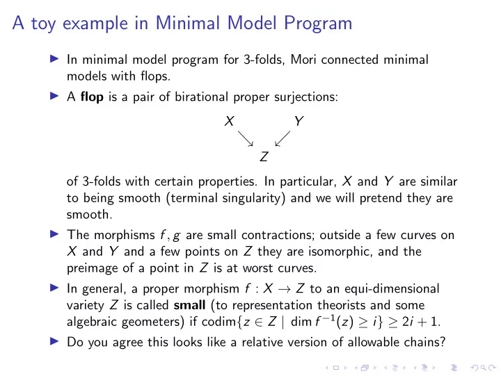
◮ In minimal model program for 3-folds, Mori connected minimal models with flops. ◮ A flop is a pair of birational proper surjections: X Y Z

• f 3-folds with certain properties. In particular, X and Y are similar

to being smooth (terminal singularity) and we will pretend they are smooth. ◮ The morphisms f , g are small contractions; outside a few curves on X and Y and a few points on Z they are isomorphic, and the preimage of a point in Z is at worst curves. ◮ In general, a proper morphism f : X → Z to an equi-dimensional variety Z is called small (to representation theorists and some algebraic geometers) if codim{z ∈ Z | dim f −1(z) ≥ i} ≥ 2i + 1. ◮ Do you agree this looks like a relative version of allowable chains?

A toy example in Minimal Model Program, cont.

codim{y ∈ Y | dim f −1(y) ≥ i} ≥ 2i + 1. Do you agree this looks like a relative version of allowable chains?

◮ It is indeed the case that the machinery of perverse sheaves is able to treat small proper morphisms as if they are smooth of dimension 0, i.e. ´ etale. ◮ Birational ´ etale morphisms are isomorphisms. For us this means we have Rf∗ICX = ICZ = Rg∗ICY . But X and Y are (almost) smooth! We have H∗(X; Q) = H∗(Z; Rf∗QX) = H∗(Z; Rf∗ICX[−3]) = H∗(Z; ICZ[−3]) = IH∗(Z; Q). ◮ Same for Y , so H∗(X; Q) = IH∗(Z; Q) = H∗(Y ; Q). ◮ For Mori, this proved that birationally equivalent minimal models in 3d have isomorphic (co)homology groups in Q-coefficients. Sweet?

Review, I

◮ Let A be your favorite abelian category. We form C(A), the abelian category of complexes of objects in A. That is, objects are X = {X n, dn

X : X n → X n+1}n∈Z with X n ∈ A and dn X ◦ dn−1 X

= 0. Morphisms are Hom(X, Y ) = {f = {f n : X n → Y n}n∈Z | f n ◦ dn−1

X

= dn−1

Y

• f n−1}.

◮ We also have K(A) as the quotient category of C(A) by modding

• ut homotopy, i.e. same objects as C(A) but two morphisms are

identified if they are homotopic, i.e. f , g : X → Y are identified if there exists h = {hn : X n → Y n−1}n∈Z such that f n − g n = hn+1 ◦ dn

X + dn−1 Y

• hn.

◮ For any complex X ∈ A one defines the cohomology Hn(X) := ker(dn

X)/ Im(dn−1 X

) ∈ A. Any morphism f : X → Y in C(A) induces a morphism of cohomology Hn(f ) : Hn(X) → Hn(Y ). Homotopic morphisms induce the same map on cohomology, so this extends to K(A).

Review, II

◮ A quasi-isomorphism is a morphism in C(A) or K(A) which induces isomorphisms on cohomology in all degrees. ◮ The derived category D(A) is the additive category whose objects are the same in C(A) and K(A), and morphisms are “X ← Y → Z” where Y → X is a quasi-isomorphism and Y → Z is a general morphism in K(A). We refer the reader to [KS,§1.6] for detail. ◮ We again have cohomology functors Hn(−) : D(A) → A for any degree n. ◮ Some useful facts:

• 1. D(A) is abelian iff A is semisimple.
• 2. Not every object X in D(A) is isomorphic to the complex of its

cohomology, that is (... → Hn−1(X) → Hn(X) → Hn+1(X) → ...) where all maps are trivial. This is the case if and only if A has homological dimension ≤ 1. In particular this is true for Ab, the category of abelian groups, but not for Sh(CP1), the sheaf of abelian groups on CP1.

Review, 2.5

Not every object X in D(A) is isomorphic to the complex of its cohomology, that is (... → Hn−1(X) → Hn(X) → Hn+1(X) → ...) where all maps are trivial. This is the case if and

• nly if A has homological dimension ≤ 1. In particular this is true for Ab, the category of abelian

groups, but not for Sh(CP1), the sheaf of abelian groups on CP1.

(This slide is not needed from the rest and may be skipped.) In fact, If X 0, Y 0 ∈ A and X, Y ∈ D(A) are the associated complexes supported only at degree 0, then HomD(A)(X, Y [n]) = Extn

A(X 0, Y 0);

• ne may prove this via an injective resolution of Y 0.

In particular, if A = Sh(CP1), and X 0 = Y 0 = QCP1, then Ext2

Sh(CP1)(X 0, Y 0) = H2(CP1; Q) = Q and we may pick a non-trivial

morphism in α ∈ HomD(A)(X, Y [2]). Let Z = M(α) be the mapping cone (see latter slides). The cohomology of Z is supported at degree −2 and −1 thanks to the long exact sequence associated to the distinguished triangle X → Y → Z → X[1], but Z is not isomorphic to its cohomology; if it is, then one may rotate the triangle to show that α = 0 and arrive at a contradiction.

Review, III

◮ For every1 X ∈ D(A), we may have truncation τ≥0(X) = Y with Y 0 = X 0/ Im d−1

X (X −1), Y n = X n for n ≥ 1 and Y n = 0 for

n ≤ −1. Likewise τ≤0(X) = Y with Y 0 = ker(d0

X : X 0 → X 1),

Y n = X n for n ≤ −1 and Y n = 0 for n ≥ 0. ◮ We have X isomorphic to τ≥0(X) iff Hn(X) = 0 for all n < 0 and likewise for τ≤0(X). Hence if X has its cohomology supported in degree from [a, b], we have X ∼ = τ≥a(τ≤b(X)) = τ≤b(τ≥a(X)) is represented by a bounded complex. ◮ This suggests a good notion of D+(A) (resp. D−(A) and Db(A)) the full subcategory of bounded below (resp. bounded above, bounded.) complexes. ◮ Also, A is the full subcategory of D(A) of those whose cohomology is supported at degree 0.

1It’s really a bad idea to write X ∈ C for some category C, as objects in a category

really form groupoid rather than a set. Cheng-Chiang is just being horribly lazy here.

Triangulated category

◮ For X ∈ C(A), the shift X[m] is the complex given by X[m]n = X m+n and dn

X[m] = (−1)mdn+m X

. ◮ The mapping cone of a morphism f : X → Y in C(A) is the complex associated to the double complex X → Y by having X n at degree (n, −1) and Y n at degree (n, 0). They come with natural morphisms Y → M(f ) and M(f ) → X[1] so that 0 → Y → M(f ) → X[1] → 0 is a short exact sequence in C(A). ◮ A triangle in C(A) is X → Y → Z → X[1] where X, Y , Z ∈ C(A) and the arrows are morphisms in C(A). This induces the same definition for K(A) and D(A). ◮ A distinguished triangle in K(A) is a triangle in K(A) that is isomorphic to some (X

f

− → Y → M(f ) → X[1]) in K(A) Likewise, a distinguished triangle is a triangle in D(A) that is isomorphic to some X

f

− → Y → M(f ) → X[1] in D(A).

Short exact sequence in the derived category?

◮ Any distinguished triangle X → Y → Z in D(A) induces a long exact sequence ... → Hn(X) → Hn(Y ) → Hn(Z) → Hn+1(X) → ... ◮ On the other hand, suppose 0 → X 0

f

− → Y 0 → Z 0 → 0 is a short exact sequence in A. Let X ∈ D(A) be the complex only at degree 0 given by X 0 and likewise for Y , Z ∈ D(A). Then there is a natural quasi-isomorphism M(f )

i

− → Z so that by putting δ(f ) := (Z

i

← − M(f ) → X[1]) we have X

f

− → Y → Z

δ(f )

− − → X[1] is a distinguished triangle. ◮ The Grothendieck group K 0(A) of A as the free abelian group generated by objects on A mod out [X 0] + [Z 0] − [Y 0] for any short exact sequence 0 → X 0 → Y 0 → Z 0 → 0 in A, and define χ(X) = (−1)n[Hn(X)] ∈ K 0(A) for any X ∈ Db(A). The one proves that a distinguished triangle X → Y → Z → X[1] again satisfy χ(X) + χ(Z) = χ(Y ).

Triangulated category

◮ We have a list of properties for distinguished triangles in K(A) and the same for D(A) (see [KS,§1.4]).

• 1. X

f

− → Y → Z → X[1] is a distinguished triangle iff Y → Z → X[1]

−f [1]

− − − → Y [1] is.

• 2. If X

id

− → X → 0 → X[1] is a distinguished triangle.

• 3. Any commutative diagram

X Y X ′ Y ′ in K(A) (resp. D(A)) can be completed to a morphism of distinguished triangles X Y Z X[1] X ′ Y ′ Z ′ X ′[1]

Triangulated category, II

We have a list of properties for distinguished triangles in K(A) and the same for D(A) (see [KS,§1.4]).

◮ Given morphisms X

f

− → Y and Y

g

− → Z. We have distinguished triangles X → Y → M(f ) → X[1], Y → Z → M(g) → Y [1] and X → Z → M(g ◦ f ) → X[1]. They should be related. The last property states:

• 4. Writing Z ′ = M(f ), X ′ = M(g) and Y ′ = M(g ◦ f ), there exists a

distinguished triangle Z ′ → Y ′ → X ′ → Z ′[1], so that these morphisms make the following diagrams commute: X Y Y Z Z ′ Y ′ Y ′ X ′ Z ′ Y ′ X[1] X ′ Y [1] Z Z ′[1] Y ′ X ′