A Study on Trajectory Optimization for the Terminal Area Keywords : - - PowerPoint PPT Presentation

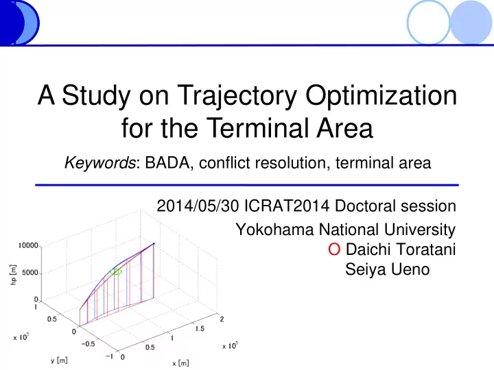
A Study on Trajectory Optimization for the Terminal Area

Keywords: BADA, conflict resolution, terminal area 2014/05/30 ICRAT2014 Doctoral session Yokohama National University O Daichi Toratani Seiya Ueno

1, Introduction

• Background and target of this study

2, Problem formulation (without conflict)

• Model of the trajectory

3, Simulation results (without conflict) 4, Problem formulation (Conflict resolution)

• Introducing conflict resolution

5, Simulation results (Conflict resolution) 6, Conclusion and future plan

Table of contents

1/25

Continuous descent operation (CDO)

1, Introduction 1/6

CDO Conventional descent operation CDO is able to improve;

• Fuel consumption
• Noise pollution

etc.

• Descending constant rate
• Constant thrust

Step-by-step Climb Descent

Tokyo international airport (Haneda airport), HND

Proposed for the CDO 2/25 Crossing

the optimal conflict-free trajectory for the CCO.

Air traffic management in the terminal area

1, Introduction 2/6

Air port Air port Conflict Fixed!

• Conventional descent operation

(Step-by-step)

• Continuous descent operation

Climb Descent Continuous climb operation (CCO)

Stepped climb CCO

3/25 The purpose of this study is …

Optimal trajectory → Arc

4/13

• Boundary conditions

𝑌0 = 90 [deg] 𝑌𝑔 = 0 [deg] 1 1 where 𝑌𝑈 = 𝜄 𝑦 𝑧 0: Initial f : Terminal

Optimal control theory and trajectory optimization

cos 𝜄 sin 𝜄

• State equation (Dubins car)

𝑒 𝑒𝑢 𝜄 𝑦 𝑧 = 𝑣 cos 𝜄 sin 𝜄 Input: 𝑣

• Criterion (Minimum input)

Minimizing 𝐾 =

𝑢0 𝑢𝑔 1

2 𝑣2 𝑒𝑢 𝑊 = 1 (const.) 𝑦 𝑧 𝜄 𝑦 𝑧

𝑌0 = 90 [deg] 𝑌𝑔 = 0 [deg] 1 1

1, Introduction 3/6

e.g.) Cruising aircraft

5/13

Related previous studies (Optimal control approach)

• A. Andreeva-Mori et al., “Scheduling of Arrival Aircraft Based on

Minimum Fuel Burn Descents”

• Fuel burn model
• Optimal trajectory

→ CDO

• J. Hu et al., “Optimal Coordinated Maneuvers for Three-Dimensional

Aircraft Conflict Resolution”

• Constraint for

conflict resolution

• Multiple aircraft

conflict resolution

• Constant velocity

1, Introduction 4/6

6/16

Problem of the trajectory optimization

1, Introduction 5/6

! It is difficult to treat spatial and temporal conflict resolutions simultaneously.

Vectoring (Spatial control) Changing velocity (Temporal control) In the practice of the air traffic control, … Spatial conflict resolution Temporal conflict resolution Slowdown Spatial and Temporal conflict resolution

?

Space-time coordinate system (STCS)

1, Introduction 6/6

t x y t = t1 t = t2 t = t3 x y

t

To develop the optimization method in the STCS.

• Conflict resolution, minimum fuel, minimum time, etc.

In the STCS,;

• The vertical axis means time.
• It is able to treat the time

along with the position.

• It is also able to calculate

the altitude. 4D trajectory Which conflict resolutions (spatial or temporal) are optimal to resolve conflict?

The target of this study is ... 7/25

• Total-energy model (TEM)

𝑈ℎ𝑠 − 𝐸 𝑊𝑈𝐵𝑇 = 𝑛𝑕0 𝑒ℎ 𝑒𝑢 + 𝑛𝑊𝑈𝐵𝑇 𝑒𝑊𝑈𝐵𝑇 𝑒𝑢 ↔ 𝑒𝑊𝑈𝐵𝑇 𝑒𝑢 = 1 𝑛 𝑈ℎ𝑠 − 𝐸 − 𝑛𝑕 sin 𝛿

• Azimuth angle

𝑒𝜔 𝑒𝑢 = 𝑕0 𝑊𝑈𝐵𝑇 tan 𝜚

• Fuel flow

𝐺𝐺 = 𝐷

𝑔1 1 + 𝑊𝑈𝐵𝑇

𝐷

𝑔2

𝑈ℎ𝑠

• Maximum climb thrust

𝑈ℎ𝑠 = 𝐷𝑈𝑑,1 1 − ℎ𝑞 𝐷𝑈𝑑,2 + 𝐷𝑈𝑑,3ℎ𝑞

2

Base of aircraft data (BADA)

γ 𝑛𝑕 𝐸 𝑀 𝑈ℎ𝑠 𝑦 ℎ𝑞

2, Problem formulation (w/o conflict) 1/5

𝜔 𝛿 𝑦 𝑧 𝐼𝑞 𝑊𝑈𝐵𝑇 8/25

• State equations

𝑒 𝑒𝑢 𝛿 𝑦 𝑧 ℎ𝑞 = 𝑕 𝑊𝑈𝐵𝑇 tan 𝜚 1 𝑛 𝑈ℎ𝑠 − 𝐸 − 𝑛𝑕 sin 𝛿 𝑞 𝑊𝑈𝐵𝑇 cos 𝛿 cos 𝜔 𝑊𝑈𝐵𝑇 cos 𝛿 sin 𝜔 𝑊𝑈𝐵𝑇 sin 𝛿

• Fuel flow

𝐺𝐺 = 𝐷

𝑔1 1 + 𝑊𝑈𝐵𝑇

𝐷

𝑔2

𝑈ℎ𝑠 𝑞: Rate of flight path angle

Base of aircraft data (BADA)

𝑊𝑈𝐵𝑇 𝜔

γ 𝑛𝑕 𝐸 𝑀 𝑈ℎ𝑠 𝑦 ℎ𝑞 𝜔 𝛿 𝑦 𝑧 𝐼𝑞 𝑊𝑈𝐵𝑇

2, Problem formulation (w/o conflict) 2/5

9/25

• State equation

𝑒 𝑒𝑡 𝜔𝑡 𝜔𝑢 𝑦 𝑧 𝑢 = 𝜆𝑡 𝜆𝑢 cos 𝜔𝑡 cos 𝜔𝑢 sin 𝜔𝑡 cos 𝜔𝑢 sin 𝜔𝑢 𝜆: Curvature Subscript 𝑡: Spatial 𝑢: Temporal Independent variable Length of the trajectory 𝑡 x y

t

𝜔𝑡 ds 𝜔𝑢 dy dx dl 𝑊 = 𝑒𝑚 𝑒𝑢 = tan 90° − 𝜔𝑤 = 1 tan 𝜔𝑢 𝑏 = − 𝜆𝑢 sin3𝜔𝑢 ↔ 𝜆𝑢 = −𝑏sin3𝜔𝑢 dl dt ds 𝜔𝑢

• Velocity and acceleration

2, Problem formulation (w/o conflict) 3/5

Space-time coordinate system (STCS)

10/25

• BADA (Independent variable: time)

𝑒 𝑒𝑢 𝜔𝑡 𝑊𝑈𝐵𝑇 𝛿 𝑦 𝑧 ℎ𝑞 = 𝑕 𝑊𝑈𝐵𝑇 tan 𝜚 1 𝑛 𝑈ℎ𝑠 − 𝐸 − 𝑛𝑕 sin 𝛿 𝑞 𝑊𝑈𝐵𝑇 cos 𝛿 cos 𝜔𝑡 𝑊𝑈𝐵𝑇 cos 𝛿 sin 𝜔𝑡 𝑊𝑈𝐵𝑇 sin 𝛿

• STCS

𝑒𝜔𝑢 𝑒𝑡 = −𝑏sin3𝜔𝑢 𝑒𝑢 𝑒𝑡 = sin 𝜔𝑢 𝑊𝑈𝐵𝑇 = 1 tan 𝜔𝑢

+

2, Problem formulation (w/o conflict) 4/5

• BADA (STCS)

𝑒 𝑒𝑡 𝜔𝑡 𝜔𝑢 𝛿 𝑦 𝑧 ℎ𝑞 𝑢 = 𝑕 sin 𝜔𝑢 tan 𝜔𝑢 tan 𝜚 −sin3𝜔𝑢 1 𝑛 𝑈ℎ𝑠 − 𝐸 − 𝑛𝑕 sin 𝛿 sin 𝜔𝑢 𝑞 cos 𝜔𝑡 cos 𝜔𝑢 cos 𝛿 sin 𝜔𝑡 cos 𝜔𝑢 cos 𝛿 cos 𝜔𝑢 sin 𝛿 sin 𝜔𝑢 11/25

Optimal control problem and calculation method

• Optimal control problem

Constraint equation Criterion Boundary conditions

𝑒𝒀 𝑒𝑡 = 𝑮 𝐾 =

𝑡𝐺

𝑀 𝑒𝑡 𝒀 𝑡0 = 𝒀𝟏 𝒀 𝑡𝑔 = 𝒀𝒈

• Two-point boundary value problem (TPBVP)

Simultaneous non-linear differential equations

• Simultaneous non-linear equations

Simultaneous non-linear equations solver

2, Problem formulation (w/o conflict) 5/5

Optimal control theory Linear approximation State equation Fuel flow Initial and terminal state

Minimizing

12/25

Optimal climbing trajectory in the 3D space

Simulation conditions

Units: 𝜔𝑡 𝑊𝑈𝐵𝑇 𝛿 𝑦 𝑧 ℎ𝑞 𝑢 = deg m/s deg m m m s 𝐺 : Terminal free Initial condition 𝜔𝑡0 𝑊𝑈𝐵𝑇0 𝛿0 𝑦0 𝑧0 ℎ𝑞0 𝑢0 = 0 150.0 5 3000

291.6 [kt] 9843 [ft]

Terminal condition 𝜔𝑡𝑔 𝑊𝑈𝐵𝑇𝑔 𝛿𝑔 𝑦𝑔 𝑧𝑔 ℎ𝑞𝑔 𝑢𝑔 = 0 250.0 𝐺 𝐺 10000 𝐺

485.0 [kt] 32808 [ft]

32808 [ft]

Data of aircraft Boeing 777-200

3, Simulation results (w/o conflict) 1/3

107.99 [nm] 54.00 [nm]

13/25

Trajectories in the 3D space and the STCS

3D space Space-time coordinate system

3, Simulation results (w/o conflict) 2/3

32808 [ft]

14/25

TAS, altitude, fuel flow, and fuel consumption

• The optimal trajectory in the STCS is derived.

39370 [ft] 583.2 [kt]

3, Simulation results (w/o conflict) 3/3

11.02 [lb/s] 6614 [lb]

700.3 [s] 2509 [kg]

15/25

Spatial conflict resolution

x y time 5 [nm] Spatial interval Vectoring (Spatial control)

Temporal conflict resolution

x y time 250 [m/s] 37.0 [s] 5 [nm] = 9260 [m] Temporal interval in the STCS Changing velocity (Temporal control)

4, Problem formulation (Conflict resolution) 1/2

16/25

If you wont to add a new constraint, … Waypoint

Interior-point constraint

4, Problem formulation (Conflict resolution) 2/2

17/25

Trajectory1 Trajectory2 Split! Initial1 Initial2 Terminal1 Terminal2 Position1 = Position2 (Specified) Angle1 = Angle2 (Free) ⋮

Interior-point constraint

4, Problem formulation (Conflict resolution) 2/2

17/25

If you wont to add a new constraint, … Waypoint Trajectory1 Trajectory2 Split! Initial1 Initial2 Terminal1 Terminal2 Position1 = Position2 (Specified) Angle1 = Angle2 (Free) ⋮ Trajectory with constraint

• The original trajectory optimization is transformed to the trajectory
• ptimization problem with a new constraint.
• To see clearly which conflict resolutions are optimal, conflict

resolution with specified point is shown.

Interior-point constraint

4, Problem formulation (Conflict resolution) 2/2

17/25

Conflict point 𝜔𝑡 𝑊𝑈𝐵𝑇 𝛿 𝑦 𝑧 ℎ𝑞 𝑢 = 0 225.9 2.410 73842 7553 384.4

439.0 [kt] 39.87 [nm] 24781 [ft]

Simulation conditions (Interior point constraint)

32808 [ft]

5, Simulation results (Conflict resolution) 1/6

54.00 [nm]

• 54.00 [nm]

107.99 [nm]

Descending aircraft Fixed

18/25

32808 [ft]

Spatial w/o conflict

Simulation conditions (Spatial conflict resolution)

5, Simulation results (Conflict resolution) 2/6

107.99 [nm] 54.00 [nm]

• 54.00 [nm]

Interior point conditions 𝜔𝑡𝑗𝑜𝑢 𝑊𝑈𝐵𝑇𝑗𝑜𝑢 𝛿𝑗𝑜𝑢 𝑦𝑗𝑜𝑢 𝑧𝑗𝑜𝑢 ℎ𝑞𝑗𝑜𝑢 𝑢𝑗𝑜𝑢 = 0 𝐺 𝐺 73842 9260 𝐺 𝐺

39.87 [nm] 5 [nm]

19/25

Spatial conflict resolution

3D space x-y plane

5, Simulation results (Conflict resolution) 3/6

Spatial w/o conflict

32808 [ft]

20/25

• It is confirmed that the spatial conflict resolution is

able to resolve the conflict with the spatial control.

Temporal w/o conflict

Simulation conditions (Temporal conflict resolution)

5, Simulation results (Conflict resolution) 4/6

54.00 [nm]

• 54.00 [nm]

107.99 [nm]

Interior point conditions 𝜔𝑡𝑗𝑜𝑢 𝑊𝑈𝐵𝑇𝑗𝑜𝑢 𝛿𝑗𝑜𝑢 𝑦𝑗𝑜𝑢 𝑧𝑗𝑜𝑢 ℎ𝑞𝑗𝑜𝑢 𝑢𝑗𝑜𝑢 = 0 𝐺 𝐺 73842 𝐺 421.4 5 [nm] / 225.9 [m/s] = 41.0 [s] 384.4 + 41.0 = 421.4 [s] Conflict point 𝑢𝑗𝑜𝑢=384.4 [s] 𝑊𝑈𝐵𝑇𝑗𝑜𝑢=225.9 [m/s] 21/25

Temporal conflict resolution

Space-time coordinate system x-y plane

5, Simulation results (Conflict resolution) 5/6

Spatial w/o conflict

22/25

• It is confirmed that the temporal conflict resolution is

able to resolve the conflict decreasing its velocity.

5, Simulation results (Conflict resolution) 6/6

Fuel flow and fuel consumption

w/o conflict Spatial Temporal Terminal time [s] 700.3 705.7 769.6 Fuel consumption [kg] [lb] 2509 2520 2581 5531 5556 5690

• The fuel consumption with the spatial conflict resolution

is lower than the fuel consumption with the temporal conflict resolution.

Cuise 𝑦𝑔 = 150000 [m] = 80.99 [nm]

11.02 [lb/s] 6614 [lb]

23/25

 The trajectory optimization method in the space-time coordinate system is developed, and the optimal trajectory is derived.  By introducing the interior-point constraint, the

• ptimal

conflict-free trajectories with spatial and temporal conflict resolutions are obtained.  The fuel consumption with the spatial conflict resolution is lower than the fuel consumption with the temporal conflict resolution.

Conclusion

6, Conclusion and future plan

24/25

 The optimal trajectories will be obtained in various boundary conditions.

• e.g.) Conflict resolution with accelerating velocity.

 The model of the trajectory will be improved.

• Introducing mass change, 𝑊

𝐷𝐵𝑇, clime rate, etc.

 Multiple aircraft will be introduced to the trajectory

• ptimization .

25/25

Future plan

6, Conclusion and future plan