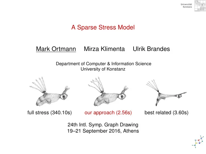
A Sparse Stress Model Mark Ortmann Mirza Klimenta Ulrik Brandes - - PowerPoint PPT Presentation

A Sparse Stress Model Mark Ortmann Mirza Klimenta Ulrik Brandes

Department of Computer & Information Science University of Konstanz

full stress (340.10s)

• ur approach (2.56s)

best related (3.60s) 24th Intl. Symp. Graph Drawing 19–21 September 2016, Athens

Full Stress Model

Goal:

◮ finding layout x = (R2)V minimizing:

s(x) =

• i,j∈(V

2)

wij(||xi − xj|| − dij)2 with

◮ dij := shortest path distances between i and j ◮ wij := 1/d2 ij

Full Stress Model

Goal:

◮ finding layout x = (R2)V minimizing:

s(x) =

• i,j∈(V

2)

wij(||xi − xj|| − dij)2 =

• i,j∈E

wij(||xi − xj|| − dij)2

• 1st term

+

• i,j∈E

wij(||xi − xj|| − dij)2

• 2nd term

with

◮ dij := shortest path distances between i and j ◮ wij := 1/d2 ij

Full Stress Model

Goal:

◮ finding layout x = (R2)V minimizing:

s(x) =

• i,j∈(V

2)

wij(||xi − xj|| − dij)2 =

• i,j∈E

wij(||xi − xj|| − dij)2

• 1st term

+

• i,j∈E

wij(||xi − xj|| − dij)2

• 2nd term

with

◮ dij := shortest path distances between i and j ◮ wij := 1/d2 ij

Complexity due to 2nd term:

◮ preprocessing: O(n(m + n log n)) ◮ time & space: O(n2)

How to deal with the 2nd Term

Related Sparse Stress Models:

◮ ignore:

◮ GRIP

(Gajer, Goodrich and Kobourov, GD’00, 2001)

◮ 1-stress

(Brandes and Pich, GD’08, 2009) ◮ replace:

◮ maxent

(Gansner, Hu and North, TVCG, 2013)

◮ COAST

(Gansner, Hu and Krishnan, GD’13, 2013) ◮ approximate shortest path matrix & set wij = 1/dij:

◮ MARS

(Khoury, Hu, Krishnan and Scheidegger, CGF, 2012)

• ur approach:

◮ approximate by term aggregation

Aggregation of Terms is an old Hat (or was it Hut)

Aggretation of terms via Barnes & Hut: (Barnes and Hut, Nature, 1986)

• 1. construct partition of V for each i ∈ V
• 2. for each partition p ∈ P(i) determine centroid
• 3. aggregation: repulsive forces only w.r.t. centroids

Result:

◮ repulsive forces: O(n log n) instead of O(n2) computations

Aggregation of Terms is an old Hat (or was it Hut)

Aggretation of terms via Barnes & Hut: (Barnes and Hut, Nature, 1986)

• 1. construct partition of V for each i ∈ V
• 2. for each partition p ∈ P(i) determine centroid
• 3. aggregation: repulsive forces only w.r.t. centroids

Result:

◮ repulsive forces: O(n log n) instead of O(n2) computations

Problem:

◮ centroids artificial nodes ⇒ no shortest-path distance

A Sparse Stress Model

Solution:

◮ select k pivots P ⊆ V ◮ assign each pivot p a partition R(p) ⊆ V with p ∈ R(p)

and R(p) ∩ R(p′) = ∅

A Sparse Stress Model

Solution:

◮ select k pivots P ⊆ V ◮ assign each pivot p a partition R(p) ⊆ V with p ∈ R(p)

and R(p) ∩ R(p′) = ∅ Our Sparse Stress Model: s′(x) =

• {i,j}∈E

wij(||xi−xj||−dij)2+

• i∈V
• p∈P\N(i)

w′

ip(||xi−xp||−dip)2,

with adapted weights w′

ij

A Sparse Stress Model - Partitioning Construction

Iterative stress minimization

(Gansner, Koren and North, GD’04, 2004):

xα

i =

• j=i wij v(i, j)
• j=i wij

with v(i, j) = xα

j +

dij(xα

i − xα j )

||xi − xj|| xj xi

v(i,j)

dij

A Sparse Stress Model - Partitioning Construction

Iterative stress minimization

(Gansner, Koren and North, GD’04, 2004):

xα

i =

• j=i wij v(i, j)
• j=i wij

with v(i, j) = xα

j +

dij(xα

i − xα j )

||xi − xj|| Each pivot aggregates terms R(p): v(i, p) ≈

• j∈R(p) wij v(i, j)
• j=i wij

xj xi

v(i,j)

dij

Requirement:

◮ dip similar to dij with j ∈ R(p) ◮ xj well distributed in close proximity around xp

Solution:

◮ assign i ∈ V to partition of closest pivot

A Sparse Stress Model - Weight Adaption

Ideal:

◮ w′ ip = j∈R(p) wij

Problem:

◮ wij’s unknown since wij = 1/d2 ij

Solution set w′

ip = s/d2 ip: ◮ s number j ∈ R(p) at least as close to p as to i

◮ s = |{j ∈ R(p) : djp ≤ dip/2}|

A Sparse Stress Model - Weight Adaption

Ideal:

◮ w′ ip = j∈R(p) wij

Problem:

◮ wij’s unknown since wij = 1/d2 ij

Solution set w′

ip = s/d2 ip: ◮ s number j ∈ R(p) at least as close to p as to i

◮ s = |{j ∈ R(p) : djp ≤ dip/2}|

Complexity of our Sparse Stress Model:

◮ preprocessing: O(k(m + n log n)) ◮ time & space: O(kn + m)

Evaluation - Setup

Data:

◮ 13 graphs 1K ≤ n ≤ 21K (Davis and Hu, Sparse Matrix Collection) ◮ 2 bipartite, 2 weighted graphs

Layout algorithms:

◮ our approach with k ∈ {50, 100, 200} pivots ◮ maxent, GRIP

, MARS, 1-stress and PivotMDS Reported results our approach:

◮ median stress layout of 25 repetitions ◮ P sampled via k-means on subset of shortest-path

distance matrix

Evaluation - Measures & Results

◮ Stress (optimally scaled) ◮ Time ◮ Procrustes Analysis ◮ Gabriel Graph Neighborhood preservation ◮ Convex Hull Classification

Evaluation - Measures & Results

◮ Stress (optimally scaled) ◮ Time ◮ Procrustes Analysis ◮ Gabriel Graph Neighborhood preservation ◮ Convex Hull Classification

Results show that our method yields:

◮ lower stress ◮ better

preservation

◮ higher similarity ◮ better

classification

◮ lower runtime

Results

graph full stress sparse 200 sparse 100 sparse 50 maxent MARS 200 MARS 100 GRIP 1-stress PivotMDS dwt1005 3elt LeHavre qh882 btree

Results

graph full stress sparse 200 sparse 100 sparse 50 maxent MARS 200 MARS 100 GRIP 1-stress PivotMDS dwt1005 3elt LeHavre qh882 btree

full stress sparse 200 maxent GRIP

Conclusion

◮ 2nd term makes full stress model too costly ◮ Sparse Stress Model: aggregation of terms

◮ preprocessing: O(k(m + n log n)) ◮ time & space: O(kn + m)

◮ proper pivot sampling and weight adaption allows

◮ better approximation ◮ less time

full stress (340.10s) our approach (2.56s) best related (3.60s)

Time Complexity

◮ Full Stress: O(n2) ◮ 1-stress: O(m) ◮ GRIP: O(nk2) with k = log max{dij : i, j ∈ V} ◮ maxent: O(m + n log n) ◮ MARS: O(kn + n log n + m) ◮ PivotMDS: O(nk) ◮ our approach: O(nk + m)

Evaluation - Data

graph n m δ(G) ∆(G) D(G) {deg(i)} {dij} dwt1005 1005 3808 3 26 34 1138bus 1138 1458 1 17 31 plat1919 1919 15240 2 18 43 3elt 4740 13722 3 9 65 USpowerGrid 4941 6594 1 19 46 commanche 7920 11880∗∗ 3 3 438.00 LeHavre 11730 15133∗∗ 1 7 33800.67 pesa 11738 33914 2 9 208 bodyy5 18589 55346 2 8 132 finance256 20657 71866 1 54 55 btree (binary tree) 1023∗ 1022 1 3 18 qh882 1764∗ 3354 1 14 32 lpship04l 2526∗ 6380 1 84 13

Sampling

• ●
• ●
• ●
• ●
• ●
• ●
• commanche

pesa 0.0225 0.0250 0.0275 0.021 0.022 0.023 0.024 50 100 150 200 50 100 150 200

number of pivots normalized stress sampling strategy

• max/min euclidean

random MIS filtration max/min sp k−means layout k−means + max/min sp max/min random sp k−means sp

• ●
• ●
• ●
• ●
• ●
• ●
• btree

USpowerGrid 0.2 0.4 0.6 0.8 0.01 0.02 0.03 0.04 50 100 150 200 50 100 150 200

number of pivots Procrustes statistic sampling strategy

• max/min euclidean

MIS filtration random k−means layout k−means + max/min sp max/min random sp max/min sp k−means sp

Results

• ur approach

related approaches graph full stress sparse 200 sparse 100 sparse 50 maxent MARS 200 MARS 100 GRIP 1-stress PivotMDS stress dwt1005 10 729 10 940 11 081 11 329 21 623 17 660 20 134 52 517 12 495 14 459 3elt 422 940 426 564 430 200 437 051 585 967 503 600 754 134 934 206 555 934 634 401 commanche 654 694 677 220 699 890 749 609 1 507 654 2 761 605 3 145 489 1 539 767 2 085 818 2 157 943 LeHavre 439 188 433 030 441 986 454 785 1 231 283 12 012 307 12 570 692 8 658 371 1 255 474 1 305 577 pesa 1 373 514 1 417 449 1 452 975 1 495 512 10 423 779 3 563 772 8 281 116 2 957 738 3 486 176 3 325 889 finance256 6 175 210 6 415 761 6 474 787 6 582 890 8 151 335 7 267 598 8 643 239 19 817 355 12 257 268 11 380 089 btree 60 206 61 839 63 325 66 122 67 871 103 436 100 767 96 235 157 988 164 329 Procrustes statistic dwt1005 0.001 0.005 0.003 0.027 0.008 0.018 0.263 0.004 0.008 3elt 0.001 0.001 0.002 0.026 0.009 0.029 0.199 0.017 0.023 commanche 0.001 0.002 0.005 0.039 0.026 0.167 0.092 0.066 0.066 LeHavre 0.001 0.001 0.001 0.012 0.163 0.173 0.256 0.010 0.010 pesa 0.009 0.010 0.010 0.095 0.025 0.070 0.017 0.021 0.021 finance256 0.009 0.006 0.005 0.013 0.007 0.018 0.206 0.042 0.041 btree 0.748 0.165 0.241 0.233 0.360 0.367 0.386 0.361 0.364 time in seconds dwt1005 1.26 0.22 0.14 0.10 0.47 1.02 2.36 0.06 0.08 0.06 3elt 31.82 0.94 0.59 0.46 2.26 16.31 8.43 0.71 0.37 0.23 commanche 340.10 4.89 2.56 1.47 3.60 22.72 12.43 2.29 0.47 0.35 LeHavre 475.05 6.53 3.48 2.37 6.31 27.57 19.50 10.18 0.81 0.54 pesa 373.23 4.25 2.47 1.53 5.96 50.10 42.68 3.56 0.95 0.60 finance256 1016.92 7.32 4.41 3.09 14.76 32.16 24.66 12.12 2.51 1.60 btree 7.79 0.38 0.15 0.10 0.63 2.70 1.48 0.06 0.06 0.03

Summary:

◮ lower stress ◮ higher similarity ◮ less time

Results

Gabriel Graph Neighborhood preservation

• ●
• ●
• ●
• ●
• ●
• ● ●
• ● ●
• ● ●
• ● ●
• ● ●
• dwt1005

LeHavre 0.00 0.25 0.50 0.75 1.00 0.00 0.25 0.50 0.75 1.00 1 2 3 4 5 1 2 3 4 5

k−neighborhood Jaccard algorithm

• GRIP

MARS 100 1−stress MARS 200 PivMDS maxent sparse 50 sparse 100 sparse 200

Convex Hull Classification

• bodyy5

finance256 0.000 0.005 0.010 0.015 0.00 0.01 0.02 0.03 0.04 1 2 3 4 5 1 2 3 4 5

k−neighborhood Error algorithm

• MARS 100

1−stress MARS 200 maxent GRIP PivMDS sparse 50 sparse 100 sparse 200 full stress

Results

graph full stress sparse 200 sparse 100 sparse 50 maxent MARS 200 MARS 100 GRIP 1-stress PivotMDS dwt1005 3elt LeHavre qh882