
SLIDE 1
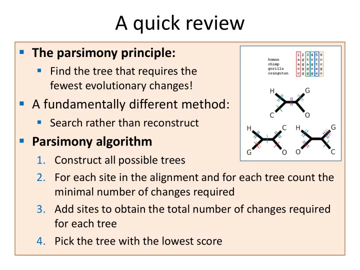
- The parsimony principle:
- Find the tree that requires the
fewest evolutionary changes!
- A fundamentally different method:
- Search rather than reconstruct
- Parsimony algorithm
- 1. Construct all possible trees
- 2. For each site in the alignment and for each tree count the
minimal number of changes required
- 3. Add sites to obtain the total number of changes required
for each tree
- 4. Pick the tree with the lowest score