A Quick Math Review Logarithms and Exponents - properties of - - PDF document

1 Analysis of Algorithms

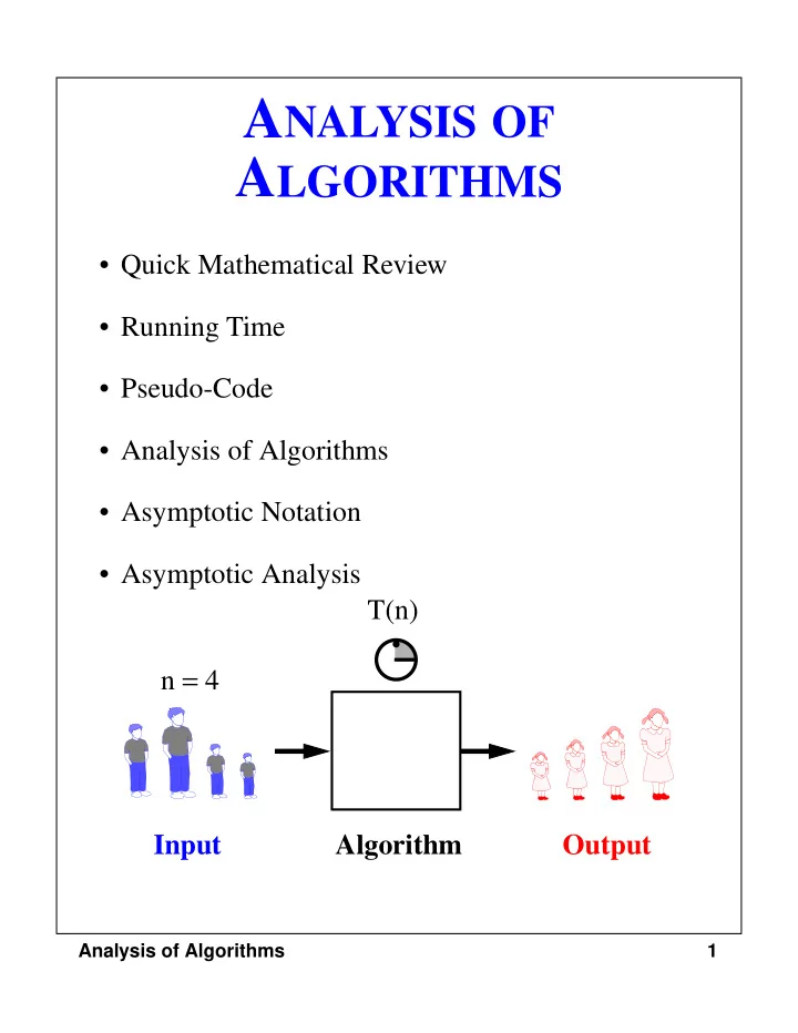
ANALYSIS OF ALGORITHMS

• Quick Mathematical Review
• Running Time
• Pseudo-Code
• Analysis of Algorithms
• Asymptotic Notation
• Asymptotic Analysis

n = 4 Algorithm Input T(n) Output

2 Analysis of Algorithms

A Quick Math Review

• Logarithms and Exponents
• properties of logarithms:

logb(xy) = logbx + logby logb(x/y) = logbx - logby logbxα = αlogbx logax logab

• properties of exponentials:

a(b+c) = abac abc = (ab)c ab/ac = a(b-c) b = a bc = a logba =

logab c*logab

3 Analysis of Algorithms

A Quick Math Review (cont.)

• Floor

x = the largest integer ≤ x

• Ceiling

x = the smallest integer x

• Summations
• general definition:
• where f is a function, s is the start index, and t is

the end index

• Geometric progression: f(i) = ai
• given an integer n 0 and a real number 0 <a ≠ 1
• geometric progressions exhibit exponential growth

f i ( )

i s = t

∑ f s ( ) f s 1 + ( ) f s 2 + ( ) … f t ( ) + + + +

=

ai 1 a a2 … an 1 an

1 +

– 1 a –

• =

+ + + + =

i = n

∑

4 Analysis of Algorithms

Average Case vs. Worst Case Running Time of an Algorithm

• An algorithm may run faster on certain data sets

than on others,

• Finding the average case can be very difficult, so

typically algorithms are measured by the worst-case time complexity.

• Also, in certain application domains (e.g., air traffic

control, surgery) knowing the worst-case time complexity is of crucial importance.

Input Instance Running Time

1 ms 2 ms 3 ms 4 ms 5 ms A B C D E F G

worst-case best-case

}

average-case

5 Analysis of Algorithms

Measuring the Running Time

• How should we measure the running time of an

algorithm?

• Experimental Study
• Write a program that implements the algorithm
• Run the program with data sets of varying size and

composition.

• Use a method like System.currentTimeMillis() to get

an accurate measure of the actual running time.

• The resulting data set should look something like:

50 100

t (ms) n

10 20 30 40 50 60

6 Analysis of Algorithms

Beyond Experimental Studies

• Experimental studies have several limitations:
• It is necessary to implement and test the algorithm

in order to determine its running time.

• Experiments can be done only on a limited set of

inputs, and may not be indicative of the running time on other inputs not included in the experiment.

• In order to compare two algorithms, the same

hardware and software environments should be used.

• We will now develop a general methodology for

analyzing the running time of algorithms that

• Uses a high-level description of the algorithm

instead of testing one of its implementations.

• Takes into account all possible inputs.
• Allows one to evaluate the efficiency of any

algorithm in a way that is independent from the hardware and software environment.

7 Analysis of Algorithms

Pseudo-Code

• Pseudo-code is a description of an algorithm that is

more structured than usual prose but less formal than a programming language.

• Example: finding the maximum element of an array.

Algorithm arrayMax(A, n): Input: An array A storing n integers. Output: The maximum element in A. currentMax ← A[0] for i ← 1 to n −1 do if currentMax < A[i] then currentMax ← A[i] return currentMax

• Pseudo-code is our preferred notation for describing

algorithms.

• However, pseudo-code hides program design issues.

8 Analysis of Algorithms

What is Pseudo-Code?

• A mixture of natural language and high-level

programming concepts that describes the main ideas behind a generic implementation of a data structure

• r algorithm.
• Expressions: use standard mathematical symbols

to describe numeric and boolean expressions

• use ← for assignment (“=” in Java)
• use = for the equality relationship (“==” in Java)
• Method Declarations:
• Algorithm name(param1, param2)
• Programming Constructs:
• decision structures:

if ... then ... [else ... ]

• while-loops:

while ... do

• repeat-loops:

repeat ... until ...

• for-loop:

for ... do

• array indexing:

A[i]

• Methods:
• calls:
• bject method(args)
• returns:

return value

9 Analysis of Algorithms

A Quick Math Review (cont.)

• Arithmetic progressions:
• An example
• two visual representations

i 1 2 3 … n + + + + =

i 1 = n

∑

n2 n + 2

• =

1 n/2 1 2 n 3 2 n+1 ... 1 2 n 1 2 n 3 3 ...

10 Analysis of Algorithms

Analysis of Algorithms

• Primitive Operations: Low-level computations that

are largely independent from the programming language and can be identified in pseudocode, e.g:

• calling a method and returning from a method
• performing an arithmetic operation (e.g. addition)
• comparing two numbers, etc.
• By inspecting the pseudo-code, we can count the

number of primitive operations executed by an algorithm.

• Example:

Algorithm arrayMax(A, n): Input: An array A storing n integers. Output: The maximum element in A. currentMax ← A[0] for i ← 1 to n −1 do if currentMax < A[i] then currentMax ← A[i] return currentMax

11 Analysis of Algorithms

Asymptotic Notation

• Goal: To simplify analysis by getting rid of

unneeded information

• Like “rounding”: 1,000,001

≈ 1,000,000

• 3n2 ≈ n2
• The “Big-Oh” Notation
• given functions f(n) and g(n), we say that

f(n) is O(g(n)) if and only if f(n) ≤ c g(n) for n n0

• c and n0 are constants, f(n) and g(n) are functions
• ver non-negative integers

Input Size Running Time cg(n) f(n) n0

12 Analysis of Algorithms

Asymptotic Notation (cont.)

• Note: Even though 7n - 3 is O(n5), it is expected that

such an approximation be of as small an order as possible.

• Simple Rule: Drop lower order terms and constant

factors.

• 7n - 3 is O(n)
• 8n2log n + 5n2 + n is O(n2log n)
• Special classes of algorithms:
• logarithmic:

O(log n)

• linear

O(n)

• quadratic

O(n2)

• polynomial

O(nk), k 1

• exponential

O(an), n> 1

• “Relatives” of the Big-Oh

− Ω(f(n)): Big Omega − Θ(f(n)): Big Theta

13 Analysis of Algorithms

Asymptotic Analysis of The Running Time

• Use the Big-Oh notation to express the number of

primitive operations executed as a function of the input size.

• For example, we say that the arrayMax algorithm

runs in O(n) time.

• Comparing the asymptotic running time
• an algorithm that runs in O(n) time is better than
• ne that runs in O(n2) time
• similarly, O(log n) is better than O(n)
• hierarchy of functions:
• log n << n << n2 << n3 << 2n
• Caution!
• Beware of very large constant factors. An

algorithm running in time 1,000,000 n is still O(n) but might be less efficient on your data set than

• ne running in time 2n2, which is O(n2)

14 Analysis of Algorithms

Example of Asymptotic Analysis

• An algorithm for computing prefix averages

Algorithm prefixAverages1(X): Input: An n-element array X of numbers. Output: An n-element array A of numbers such that A[i] is the average of elements X[0], ... , X[i]. Let A be an array of n numbers. for i ← 0 to n - 1 do a ← 0 for j ← 0 to i do a ← a + X[j] A[i] ← a/(i + 1) return array A

• Analysis ...

15 Analysis of Algorithms

Example of Asymptotic Analysis

• A better algorithm for computing prefix averages:

Algorithm prefixAverages2(X): Input: An n-element array X of numbers. Output: An n-element array A of numbers such that A[i] is the average of elements X[0], ... , X[i]. Let A be an array of n numbers. s ← 0 for i ← 0 to n - 1 do s ← s + X[i] A[i] ← s/(i + 1) return array A

• Analysis ...

16 Analysis of Algorithms

Advanced Topics: Simple Justification Techniques

• By Example
• Find an example
• Find a counter example
• The “Contra” Attack
• Find a contradiction in the negative statement
• Contrapositive
• Induction and Loop-Invariants
• Induction
• 1) Prove the base case
• 2) Prove that any case n implies the next case (n + 1) is also true
• Loop invariants
• Prove initial claim S0
• Show that Si-1 implies Si will be true after iteration i

17 Analysis of Algorithms

Advanced Topics: Other Justification Techniques

• Proof by Excessive Waving of Hands
• Proof by Incomprehensible Diagram
• Proof by Very Large Bribes
• see instructor after class
• Proof by Violent Metaphor
• Don’t argue with anyone who always assumes a

sequence consists of hand grenades

• The Emperor’s New Clothes Method
• “This proof is so obvious only an idiot wouldn’t be

able to understand it.”